Table of Contents
Warning
This document is in the process of being converted to DocBook.
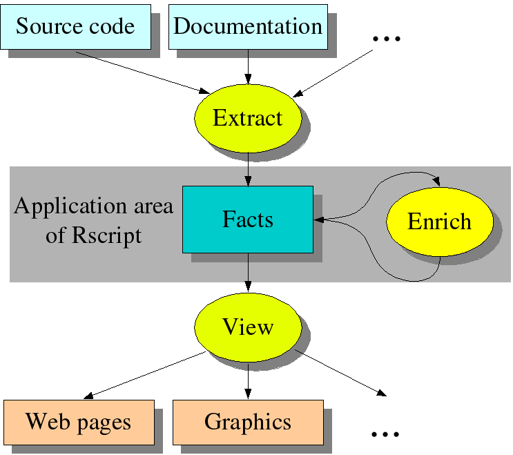
Extract-Enrich-View paradigm. Rscript is a small scripting language based on the relational calculus. It is intended for analyzing and querying the source code of software systems: from finding uninitialized variables in a single program to formulating queries about the architecture of a complete software system. Rscript fits well in the extract-enrich-view paradigm shown in Figure 1.1, “The extract-enrich-view paradigm”.
Extract. Given the source text, extract relevant information from it in the form of relations. Examples are the CALLS relation that describes direct calls between procedures, the USE relation that relates statements with the variables that are used in the statements, and the PRED relation that relates a statement with its predecessors in the control flow graph. The extraction phase is outside the scope of Rscript but may, for instance, be implemented using ASF+SDF and we will give examples how to do this.
Enrich. Derive additional information from the relations extracted from the source text. For instance, use CALLS to compute procedures that can also call each other indirectly (using transitive closure). Here is where Rscript shines.
View. The result of the enrichment phase are again bags and relations. These can be displayed with various tools like, Dot [KN96], Rigi [MK88] and others. Rscript is not concerned with viewing but we will give some examples anyway.
Application of Relations to Program Analysis. Many algorithms for program analysis are usually presented as graph algorithms and this seems to be at odds with the extensive experience of using term rewriting for tasks as type checking, fact extraction, analysis and transformation. The major obstacle is that graphs can and terms cannot contain cycles. Fortunately, every graph can be represented as a relation and it is therefore natural to have a look at the combination of relations and term rewriting. Once you start considering problems from a relational perspective, elegant and concise solutions start to appear. Some examples are:
-
Analysis of call graphs and the structure of software architectures.
-
Detailed analysis of the control flow or dataflow of programs.
-
Program slicing.
-
Type checking.
-
Constraint problems.
What's new in Rscript? Given the considerable amount of related work to be discussed below, it is necessary to clearly establish what is and what is not new in our approach:
-
We use sets and relations like Rigi [MK88] and GROK [Hol96] do. After extensive experimentation we have decided not to use bags and multi-relations like in RPA [FKO98].
-
Unlike several other systems we allow nested sets and relations and also support
n-ary relations as opposed to just binary relations but don't support the complete repertoire ofn-ary relations as in SQL. -
We offer a strongly typed language with user-defined types.
-
Unlike Rigi [MK88], GROK [Hol96] and RPA [FKO98]we provide a relational calculus as opposed to a relational algebra. Although the two have the same expressive power, a calculus increases, in our opinion, the readability of relational expressions because they allow the introduction of variables to express intermediate results.
-
We integrate an equation solver in a relational language. In this way dataflow problems can be expressed.
-
We introduce an location datatype with associated operations to easily manipulate references to source code.
-
There is some innovation in syntactic notation and specific built-in functions.
-
We introduce the notion of an Rstore that generalizes the RSF tuple format of Rigi. An Rstore consists of name/value pairs, where the values may be arbitrary nested bags or relations. An Rstore is a language-independent exchange format and can be used to exchange complex relational data between programs written in different languages.
Suppose a mystery box ends up on your desk. When you open it, it contains a huge software system with several questions attached to it:
-
How many procedure calls occur in this system?
-
How many procedures contains it?
-
What are the entry points for this system, i.e., procedures that call others but are not called themselves?
-
What are the leaves of this application, i.e., procedures that are called but do not make any calls themselves?
-
Which procedures call each other indirectly?
-
Which procedures are called directly or indirectly from each entry point?
-
Which procedures are called from all entry points?
There are now two possibilities. Either you have this superb programming environment or tool suite that can immediately answer all these questions for you or you can use Rscript.
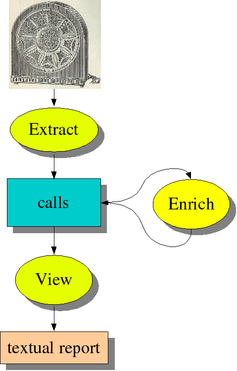
To illustrate this process consider the workflow in Figure 1.2, “Workflow for analyzing mystery box”. First we have to extract the calls
from the source code. Recall that Rscript does not consider fact
extraction per se so we assume that this call graph
has been extracted from the software by some other tool. Also keep in
mind that a real call graph of a real application will contain thousands
and thousands of calls. Drawing it in the way we do later on in Figure 1.3, “Graphical representation of the calls
relation” makes no sense since we get a uniformly black
picture due to all the call dependencies. After the extraction phase, we
try to understand the extracted facts by writing queries to explore
their properties. For instance, we may want to know how many
calls there are, or how many procedures.
We may also want to enrich these facts, for instance, by computing who
calls who in more than one step. Finally, we produce a simple textual
report giving answers to the questions we are interested in.
Figure 1.2. Workflow for analyzing mystery box
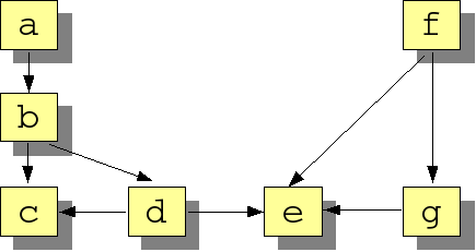
Now consider the call graph shown in Figure 1.3, “Graphical representation of the calls
relation”. This section is intended to give you a
first impression what can be done with Rscript. Please return to
this example when you have digested the detailed description of
Rscript in the section called “The Rscript Language”, the section called “Built-in Operators” and the section called “Built-in Functions”.
Rscript supports some basic data types like integers and strings
which are sufficient to formulate and answer the questions at hand.
However, we can gain readability by introducing separately named types
for the items we are describing. First, we introduce therefore a new
type proc (an alias for strings) to denote
procedures:
type proc = str
Suppose that the following facts have been extracted from the
source code and are represented by the relation
Calls:
rel[proc , proc] Calls =
   { <"a", "b">, <"b", "c">, <"b", "d">, <"d", "c">, <"d","e">,
     <"f", "e">, <"f", "g">, <"g", "e">
   }
This concludes the preparatory steps and now we move on to answer the questions.
To determine the numbers of calls, we simply determine the
number of tuples in the Calls relation, as
follows:
int nCalls = # Calls
The
operator # determines the number of elements in a
set or relation and is explained in the section called “Miscellaneous”. In this example,
nCalls will get the value
8.
We get the number of procedures by determining which names occur
in the tuples in the relation Calls and then
determining the number of names:
set[proc] procs = carrier(Calls)
int nprocs = # procs
The built-in function carrier determines all
the values that occur in the tuples of a relation. In this case,
procs will get the value {"a", "b", "c",
"d", "e", "f", "g"} and nprocs will thus
get value 7. A more concise way of expressing this
would be to combine both steps:
int nprocs = # carrier(Calls)
The next step in the analysis is to determine which
entry points this application has, i.e.,
procedures which call others but are not called themselves. Entry
points are useful since they define the external interface of a system
and may also be used as guidance to split a system in parts. The
top of a relation contains those left-hand sides of
tuples in a relation that do not occur in any right-hand side. When a
relation is viewed as a graph, its top corresponds to the root nodes
of that graph. Similarly, the bottom of a relation
corresponds to the leaf nodes of the graph. See the section called “Bottom of a Relation: bottom” for more details. Using
this knowledge, the entry points can be computed by determining the
top of the Calls relation:
set[proc] entryPoints = top(Calls)
In this case, entryPoints is equal to
{"a", "f"}. In other words, procedures
"a" and "f" are the entry points
of this application.
In a similar spirit, we can determine the leaves of this application, i.e., procedures that are being called but do not make any calls themselves:
set[proc] bottomCalls = bottom(Calls)
In this case, bottomCalls is equal to
{"c", "e"}.
We can also determine the indirect calls
between procedures, by taking the transitive closure of the
Calls relation:
rel[proc, proc] closureCalls = Calls+
In this case, closureCalls is equal to
{<"a", "b">, <"b", "c">, <"b", "d">, <"d", "c">, <"d","e">,
 <"f", "e">, <"f", "g">, <"g", "e">, <"a", "c">, <"a", "d">,
 <"b", "e">, <"a", "e">
}
We know now the entry points for this application ("a"
and "f") and the indirect call relations.
Combining this information, we can determine which procedures are
called from each entry point. This is done by taking the
right image of closureCalls.
The right image operator determines yields all right-hand sides of
tuples that have a given value as left-hand side:
set[proc] calledFromA = closureCalls["a"]
yields {"b", "c", "d", "e"} and
set[proc] calledFromF = closureCalls["f"]
yields {"e", "g"}.
Finally, we can determine which procedures are called from both
entry points by taking the intersection of the two sets
calledFromA and
calledFromF
set[proc] commonProcs = calledFromA inter calledFromF
which yields {"e"}. In other words, the
procedures called from both entry points are mostly disjoint except
for the common procedure "e".
These findings can be verified by inspecting a graph view of the
calls relation as shown in Figure 1.3, “Graphical representation of the calls
relation”. Such a
visual inspection does not scale very well to
large graphs and this makes the above form of analysis particularly
suited for studying large systems.
Rscript is based on binary relations only and
has no direct support for n-ary relations with
labeled columns as usual in a general database language. However, some
syntactic support for n-ary relations exists.
We will explain this further below. An Rscript consists of a sequence of
declarations for variables and/or functions. Usually, the value of one of
these variables is what the writer of the script is interested in. The
language has scalar types (Boolean, integer, string, location) and
composite types (set and relation). Expressions are constructed from
comprehensions, function invocations and operators. These are all
described below.}
Booleans.
The Booleans are represented by the type
bool and have two values: true
and false.
Integers.
The integer values are represented by the type
int and are written as usual, e.g.,
0, 1, or
123.
Strings.
The string values are represented by the type
str and consist of character sequences surrounded
by double quotes. e.g., "a" or "a\ long\
string".
Locations.
Location values are represented by the type
loc and serve as text coordinates in a specific
source file. They should always be generated
automatically but for the curious here is an example how they look
like: area-in-file("/home/paulk/example.pico", area(6, 17,
6, 18, 131, 1)).
Tuples.
Tuples are represented by the type
<T1,
T2>,
where T1 and
T2 are arbitrary
types. An example of a tuple type is <int,
str>. Rscript directly supports tuples consisting of two
elements (also know as pairs). For convenience,
n-ary tuples are also allowed, but there
are some restrictions on their use, see the paragraph Relations below.
Examples are:
-
<1, 2>is of type<int, int>, -
<1, 2, 3>is of type<int, int, int>, -
<1, "a", 3>is of type<int, str, int>,
Sets.
Sets are represented by the type
set[T],
where T is an arbitrary type. Examples are
set[int], set[<int,int>]
and set[set[str]]. Sets are denoted by a list of
elements, separated by comma's and enclosed in braces as in
{E1,
E2,
...,
En},
where the
En
(1 <= i <=
n) are expressions that yield the desired
element type. For example,
-
{1, 2, 3}is of typeset[int], -
{<1,10>, <2,20>, <3,30>}is of typeset[<int,int>], -
{<"a",10>, <"b",20>,
          <"c",30>}
is of typeset[<str,int>], and -
{{"a", "b"}, {"c", "d", "e"}}is of typeset[set[str]].
Relations.
Relations are nothing more than sets of tuples, but since they
are used so often we provide some shorthand notation for them.
Relations are represented by the type
rel[,
where
T1,T2]T1T2 are arbitrary
types; it is a shorthand for
set[<.
Examples are T1,
T2>]rel[int,str] and
rel[int,set[str]]. Relations are denoted by
{<E11,
E12>,
<E21,
E22>,
...,
<En1,
En2>},
where the
Eij
are expressions that yield the desired element type. For example,
{<1, "a">, <2, "b">, <3,"c">} is
of type rel[int, str]. Not surprisingly,
n-ary relations are represented by the type
rel[
which is a shorthand for
T1,
T2, ...,
Tn]set[<.
Most built-in operators and functions require binary relations as
arguments. It is, however, perfectly possible to use
T1,
T2, ...,
Tn>]n-ary relations as values, or as arguments
or results of functions. Examples are:
-
{<1,10>, <2,20>, <3,30>}is of typerel[int,int](yes indeed, you saw this same example before and then we gaveset[<int,int>]as its type; remember that these types are interchangeable.), -
{<"a",10>, <"b",20>,
          <"c",30>}
is of typerel[str,int], and -
{{"a", 1, "b"}, {"c", 2, "d"}}is of typerel[str,int,str].
Alias types. Everything can be expressed using the elementary types and values that are provided by Rscript. However, for the purpose of documentation and readability it is sometimes better to use a descriptive name as type indication, rather than an elementary type. The type declaration
typeT1 =T2
states that the new type name
T1 can be used
everywhere instead of the already defined type name
T2. For
instance,
type ModuleId = str
type Frequency = int
introduces two new type names ModuleId and
Frequency, both an alias for the type
str. The use of type aliases is a good way to hide
representation details.
Composite Types and Values. In ordinary programming languages record types or classes exist to introduce a new type name for a collection of related, named, values and to provide access to the elements of such a collection through their name. In Rscript, tuples with named elements provide this facility. The type declaration
type T = <T1F1 ,...,TnFn>
introduces a new composite type T,
with n elements. The
i-th
elementTi
Fi
has type
Ti
and field name
Fi.
The common dot notation for field access is used to address an element
of a composite type. If V is a variable of
type T, then the
i-th element can be accessed by
V.Fi.
For instance,\footnote{The variable declarations that appear on lines
2 and 3 of this example are explained fully in the section called “Declarations”.
type Triple = <int left, str middle, bool right>
Triple TR = <3, "a", true>
str S = TR.middle
first introduces the composite type Triple
and defines the Triple variable
TR. Next, the field selection
TR.middle is used to define the string
S.
Implementation Note. The current implementation severely restricts the re-use of field names in different type declarations. The only re-use that is allowed are fields with the same name and the same type that appear at the same position in different type declarations.
Type Equivalence.
An Rscript should be well-typed, this
means above all that identifiers that are used in expressions have
been declared, and that operations and functions should have
operands of the required type. We use structural
equivalence between types as criterion for type equality.
The equivalence of two types
T1 and
T2 can be
determined as follows:
-
Replace in both
T1 andT2 all user-defined types by their definition until all user-defined types have been eliminated. This may require repeated replacements. This gives, respectively,T1' andT2'. -
If
T1' andT2' are identical, thenT1 andT2 are equal. -
Otherwise
T1 andT2 are not equal.
We will use the familiar notation
{E1, ..., Em | G1, ..., Gn}
to denote the construction of a set consisting of the union of
successive values of the expressions
E1 ,...,
Em.
The values and the generated set are determined by
E1 ,...,
Em
and the generators
G1 ,...,
Gn.
E is computed for all possible combinations
of values produced by the generators. Each generator may introduce new
variables that can be used in subsequent generators as well as in the
expressions E1 ,...,
Em.
A generator can use the variables introduced by preceding generators.
Generators may enumerate all the values in a set or relation, they may
perform a test, or they may assign a value to variables.
Enumerator. Enumerators generate all the values in a given set or relation. They come in two flavors:
-
TV:E: the elements of the setS(of typeset[) that results from the evaluation of expressionT]Eare enumerated and subsequently assigned to the new variableVof typeT. Examples are:-
int N : {1, 2, 3, 4, 5}, -
str K : KEYWORDS, whereKEYWORDSshould evaluate to a value ofset[str].
-
-
<: the elements of the relationD1, ...,Dn> :ER(of typerel[T'1,...,T'n], whereT'iis determined by the type of each targetDi, see below) that results from the evaluation of expressionEare enumerated. Thei-the element (i=1,...,n) of the resultingn-tuple is subsequently combined with each targetDias follows:-
If
Diis a variable declaration of the formTiVi, then thei-th element is assigned toVi. -
If
Diis an arbitrary expressionEi, then the value of thei-th element should be equal to the value ofEi. If they are unequal, computation continues with enumerating the next tuple in the relationR.
Examples are:
-
<str K, int N> : {<"a",10>,
                <"b",20>, <"c",30>}
. -
<str K, int N> : FREQUENCIES, whereFREQUENCIESshould evaluate to a value of typerel[str,int]. -
<str K, 10> : FREQUENCIES, will only generate pairs with10as second element.
-
Test.
A test is a boolean-valued expression. If the evaluation
yields true this indicates that the current
combination of generated values up to this test is still as desired
and execution continues with subsequent generators. If the
evaluation yields false this indicates that the
current combination of values is undesired, and that another
combination should be tried. Examples:
-
N >= 3tests whetherNhas a value greater than or equal3. -
S == "coffee"tests whetherSis equal to the string"coffee".
In both examples, the variable (N,
respectively, S) should have been introduced by a
generator that occurs earlier in the enclosing comprehension.
Assignment. Assignments assign a value to one or more variables and also come in two flavors:
-
TV<-EEto the new variableVof typeT. -
<: combines the elements of theR1, ...,Rn> <-En-tuple resulting from the evaluation of expressionEwith eachTias follows:-
If
Riis a variable declaration of the formTiVii-th element is assigned toVi -
If
Riis an arbitrary expressionEi, then the value of thei-th element should be equal to the value ofEi. If they are unequal, the assignment acts as a test that fails (see above).
-
Examples of assignments are:
-
rel[str,str] ALLCALLS <- CALLS+assigns the transitive closure of the relationCALLSto the variableALLCALLS. -
bool Smaller <- A <= Bassigns the result of the testA <= Bto the Boolean variableSmaller. -
<int N, str S, 10> <- Eevaluates expressionE(which should yield a tuple of type<int, str, int>) and performs a tuple-wise assignment to the new variablesNandSprovided that the third element of the result is equal to10. Otherwise the assignment acts as a test that fails.
-
{X | int X : {1, 2, 3, 4, 5}, X >= 3}yields the set{3,4,5}. -
{<X, Y> | int X : {1, 2, 3}, int Y : {2, 3, 4}, X >= Y}yields the relation{<2, 2>, <3, 2>, <3, 3>}. -
{<Y, X> | <int X, int Y> : {<1,10>, <2,20>}}yields the inverse of the given relation:{<10,1>, <20,2>}. -
{X, X * X | X : {1, 2, 3, 4, 5}, X >= 3}yields the set{3,4,5,9,16,25}.
A variable declaration has the form
TV=E
where T is a type,
V is a variable name, and
E is an expression that should have type
T. The effect is that the value of
expression E is assigned to
V and can be used later on as
V's value. Double declarations are not
allowed. As a convenience, also declarations without an initialization
expression are permitted and have the form
TV
and
only introduce the variable V.
Examples:
-
int max = 100declares the integer variablemaxwith value100. -
The definition
rel[str,int] day = {<"mon", 1>, <"tue", 2>, <"wed",3>, <"thu", 4>, <"fri", 5>, <"sat",6>, <"sun",7>}declares the variable
day, a relation that maps strings to integers.
Local variables can be introduced as follows:
Ewhere1TV1 =E1, ...,TnVn=Enend where
First
the local variables
Vi
are bound to their respective values
Ei,
and then the value of expression E is
yielded.
A function declaration has the form
TF(1TV1, ...,TnVn) =E
Here
T is the result type of the function and
this should be equal to the type of the associated expression
E. Each
Ti
                Vi
represents a typed formal parameter of the function. The formal
parameters may occur in E and get their
value when F is invoked from another
expression. Example:
-
The function declaration
rel[int, int] invert(rel[int,int] R) =
   {<Y, X> | <int X, int Y> : R }
yields the inverse of the argument relation R. For instance,
invert({<1,10>, <2,20>})yields{<10,1>, <20,2>}.
Parameterized types in function declarations.
The types that occur in function declarations may also contain
type variables that are written as
& followed by an identifier. In this way
functions can be defined for arbitrary types. Examples:
-
The declaration
rel[&T2, &T1] invert2(rel[&T1,&T2] R) =
   {<Y, X> | <&T1 X, &T2 Y> : R }
yields an inversion function that is applicable to any binary relation. For instance,
-
invert2({<1,10>, <2,20>})yields{<10,1>, <20,2>}, -
invert2({<"mon", 1>, <"tue", 2>})yields{<1, "mon">, <2, "tue">}.
-
-
The function
<&T2, &T1> swap(&T1 A, &T2 B) = <B, A>
can be used to swap the elements of pairs of arbitrary types. For instance,
-
swap(<1, 2>)yields<2,1>and -
swap(<"wed", 3>)yields<3, "wed">.
-
An assert statement may occur everywhere where a declaration is allowed. It has the form
assertL:E
where
L is a string that serves as a label for
this assertion, and E is a boolean-value
expression. During execution, a list of true and false assertions is
maintained. When the script is executed as a test
suite a summary of this information is shown to the user.
When the script is executed in the standard fashion, the assert
statement has no affect. Example:
-
assert "Equality on Sets 1": {1, 2, 3, 1} == {3, 2, 1, 1}
It is also possible to define mutually dependent sets of equations:
equations
initial
TV1 init I1
...
Tn Vn init In
satisfy
V1 = E1
...
Vn = En
end equations
In the initial section, the variables
Vi
are declared and initialized. In the satisfy
section, the actual set of equations is given. The expressions
Ei
may refer to any of the variables
Vi
(and to any variables declared earlier). This set of equations is
solved by evaluating the expressions
Ei,
assigning their value to the corresponding variables
Vi,
and repeating this as long as the value of one of the variables was
changed. This is typically used for solving a set of dataflow
equations. Example:
-
Although transitive closure is provided as a built-in operator, we can use equations to define the transitive closure of a relation. Recall that \[R+ = R \cup (R \circ R) \cup (R \circ R \circ R) \cup ... .\] This can be expressed as follows.
Warning
Fix expression.
rel[int,int] R =  {<1,2>, <2,3>, <3,4>}

equations
  initial
     rel[int,int] T init R
  satisfy
     T = T union (T o R)
end equations
The resulting value of
Tis as expected:{<1,2>, <2,3>, <3,4>, <1, 3>, <2, 4>, <1, 4>}
The built-in operators can be subdivided in several broad categories:
-
Operations on Booleans (the section called “Operations on Booleans”): logical operators (
and,or,impliesandnot). -
Operations on integers (the section called “Operations on Integers”): arithmetic operators (
+,-,*, and/) and comparison operators (==,!=,<,<=,>, and>=). -
Operations on strings (the section called “Operations on Strings”): comparison operators (
==,!=,<,<=,>, and>=). -
Operations on locations (the section called “Operations on Locations”). comparison operators (
==,!=,<,<=,>, and>=). -
Operations on sets or relations (the section called “Operations on Sets or Relations”): membership tests (
in,notin), comparison operators (==,!=,<,<=,>, and>=), and construction operators (union,inter,diff). -
Operations on relations (the section called “Operations on Relations”): composition (
o), Cartesian product (x), left and right image operators, and transitive closures (+,*).
The following sections give detailed descriptions and examples of all built-in operators.
Table 1.1. Operations on Booleans
| Operator | Description |
|---|---|
bool1
and
bool2 | yields true if both arguments have the
value true and false otherwise |
bool1
and
bool2 | yields true if either argument has the
value true and false otherwise |
bool1
implies
bool2 | yields false if
bool1 has the
value true and
bool2 has
value false, and true
otherwise |
not
bool | yields true if bool is false and true otherwise |
Table 1.2. Operations on Integers
| Operator | Description |
|---|---|
int1
==
int2 | yields true if both arguments are
numerically equal and false otherwise |
int1
!=
int2 | yields true if both arguments are
numerically unequal and false
otherwise |
int1
<=
int2 | yields true if
int1 is
numerically less than or equal to
int2 and
false otherwise |
int1
<
int2 | yields true if
int1 is
numerically less than
int2 and
false otherwise |
int1
>=
int2 | yields true if
int1 is
numerically greater than or equal than
int2 and
false otherwise |
int1
>
int2 | yields true if
int1 is
numerically greater than
int2 and
false otherwise |
int1
+
int2 | yields the arithmetic sum of
int1 and
int2 |
int1
-
int2 | yields the arithmetic difference of
int1 and
int2 |
int1
*
int2 | yields the arithmetic product of
int1 and
int2 |
int1
/
int2 | yields the arithmetic division of
int1 and
int2 |
Table 1.3. Operations on Strings
| Operator | Description |
|---|---|
str1
==
str2 | yields true if both arguments are
equal and false otherwise |
str1
!=
str2 | yields true if both arguments are
unequal and false otherwise |
str1
<=
str2 | yields true if
str1 is
lexicographically less than or equal to
str2 and
false otherwise |
str1
<
str2 | yields true if
str1 is
lexicographically less than
str2 and
false otherwise |
str1
>=
str2 | yields true if
str1 is
lexicographically greater than or equal to
str2 and
false otherwise |
str1
>
str2 | yields true if
str1 is
lexicographically greater than
str2 and
false otherwise |
Table 1.4. Operations on Locations
| Operator | Description |
|---|---|
loc1
==
loc2 | yields true if both arguments are
identical and false otherwise |
loc1
!=
loc2 | yields true if both arguments are not
identical and false otherwise |
loc1
<=
loc2 | yields true if
loc1 is
textually contained in or equal to
loc2 and
false otherwise |
loc1
<
loc2 | yields true if
loc1 is
strictly textually contained in
loc2 and
false otherwise |
loc1
>=
loc2 | yields true if
loc1 is
textually encloses or is equal to
loc2 and
false otherwise |
loc1
>=
loc2 | yields true if
loc1 is
textually encloses
loc2 and
false otherwise |
Examples.
In the following examples the offset and length part of a
location are set to 0; they are not used when
determining the outcome of the comparison operators.
-
area-in-file("f", area(11, 1, 11, 9, 0, 0)) < area-in-file("f", area(10, 2, 12, 8, 0, 0))yieldstrue. -
area-in-file("f", area(10, 3, 11, 7, 0,0)) < area-in-file("f", area(10, 2, 11, 8, 0, 0))yieldstrue. -
area-in-file("f", area(10, 3, 11, 7, 0, 0)) < area-in-file("g", area(10, 3, 11, 7, 0, 0))yieldsfalse.
Table 1.5. Membership Tests
| Operator | Description |
|---|---|
any in
set | yields true if
any occurs as element in
set and false
otherwise |
any notin
set | yields false if
any occurs as element in
set and false
otherwise |
tuple in
rel | yields true if
tuple occurs as element in
rel and false
otherwise |
tuple
notin
rel | yields false if
tuple occurs as element in
rel and false
otherwise |
Examples.
-
3 in {1, 2, 3}yieldstrue. -
4 in {1, 2, 3} yields
false. -
3 notin {1, 2, 3}yieldsfalse. -
4 notin {1, 2, 3}yieldstrue. -
<2,20> in {<1,10>, <2,20>, <3,30>}yieldstrue. -
<4,40> notin {<1,10>, <2,20>, <3,30>}yieldstrue.
Note.
If the first argument of these operators has type
T, then the second argument should have
type set[.
T]
Table 1.6. Comparisons
| Operator | Description |
|---|---|
set1
==
set2 | yields true if both arguments are
equal sets and false otherwise |
set1
!=
set2 | yields true if both arguments are
unequal sets and false otherwise |
set1
<=
set2 | yields true if
set1 is a
subset of
set2 and
false otherwise |
set1
<
set2 | yields true if
set1 is a
strict subset of
set2 and
false otherwise |
set1
>=
set2 | yields true if
set1 is a
superset of
set2 and
false otherwise |
set1
>
set2 | Yields true if
set1 is a
strict superset of
set2 and
false otherwise |
Table 1.7. Construction
| Operator | Description |
|---|---|
set1
union
set2 | yields the set resulting from the union of the two arguments |
set1
inter
set2 | yields the set resulting from the intersection of the two arguments |
set1
\
set2 | yields the set resulting from the difference of the two arguments |
Examples.
-
{1, 2, 3} union {4, 5, 6}yields{1, 2, 3, 4, 5, 6}. -
{1, 2, 3} union {1, 2, 3}yields{1, 2, 3}. -
{1, 2, 3} union {4, 5, 6}yields{1, 2, 3, 4, 5, 6}. -
{1, 2, 3} inter {4, 5, 6}yields{ }. -
{1, 2, 3} inter {1, 2, 3}yields{1, 2, 3}. -
{1, 2, 3, 4} \ {1, 2, 3}yields{4}. -
{1, 2, 3} \ {4, 5, 6}yields{1, 2, 3}.
Table 1.9. Operations on Relations
| Operator | Description |
|---|---|
rel1
o
rel2 | yields the relation resulting from the composition of the two arguments |
set1
x
set2 | yields the relation resulting from the Cartesian product of the two arguments |
rel [-,
set ] | yields the left image of
rel |
rel [-,
elem ] | yields the left image of
rel |
rel [
set , -] | yields the right image of
rel |
rel [
elem , -] | yields the right image of
rel |
rel [
elem ] | yields the right image of
rel |
rel [
set ] | yields the right image of
rel |
rel
+ | yields the relation resulting from the transitive closure
of rel |
rel
* | yields the relation resulting from the reflexive
transitive closure of rel |
Composition: o.
The composition operator combines two relations and can be
defined as follows:
rel[&T1,&T3] compose(rel[&T1,&T2] R1, rel[&T2,&T3] R2) =
   {<V, Y> | <&T1 V, &T2 W> : R1, <&T2 X, &T3 Y> : R2, W == X }
Example.
-
{<1,10>, <2,20>, <3,15>} o {<10,100>, <20,200>}yields{<1,100>, <2,200>}.
Carthesian product: x.
The product operator combines two sets into a relation and can
be defined as follows:
rel[&T1,&T2] product(set[&T1] S1, set[&T2] S2) =
   {<V, W> | &T1 V : S1, &T2 W : S2 }
Example.
-
{1, 2, 3} x {9}yields{<1, 9>, <2, 9>, <3, 9>}.
Left image: [-, ].
Taking the left image of a relation amounts to selecting some
elements from the domain of a relation. The left
image operator takes a relation and an element
E and produces a set consisting of all
elements
Ei
in the domain of the relation that occur in tuples of the form
<. It can be defined as
follows:Ei,
E>
set[&T1] left-image(rel[&T1,&T2] R, &T2 E) =
   { V | <&T1 V, &T2 W> : R, W == E }
The left image operator can be extended to take a set of elements as second element instead of a single element:
set[&T1] left-image(rel[&T1,&T2] R, set[&T2] S) =
   { V | <&T1 V, &T2 W> : R, W in S }
Examples.
Assume that Rel has value
{<1,10>, <2,20>, <1,11>, <3,30>,
        <2,21>}
in the following examples.
-
Rel[-,10]yields{1}. -
Rel[-,{10}]yields{1}. -
Rel[-,{10, 20}]yields{1, 2}.
Right image: [ ] and [
,-].
Taking the right image of a relation amounts to selecting some
elements from the range of a relation. The right
image operator takes a relation and an element
E and produces a set consisting of all
elements
Ei
in the range of the relation that occur in tuples of the form
<. It can be defined as follows:E,
Ei
>
set[&T2] right-image(rel[&T1,&T2] R, &T1 E) =
   { W | <&T1 V, &T2 W> : R, V == E }
The right image operator can be extended to take a set of elements as second element instead of a single element:
set[&T2] right-image(rel[&T1,&T2] R, set[&T1] S) =
   { W | <&T1 V, &T2 W> : R, V in S}
Examples.
Assume that Rel has value
{<1,10>, <2,20>, <1,11>, <3,30>,
        <2,21>}
in the following examples.
-
Rel[1]yields{10, 11}. -
Rel[{1}]yields {10, 11}. -
Rel[{1, 2}]yields{10, 11, 20, 21}.
These expressions are abbreviations for, respectively
Rel[1,-], Rel[{1},-], and
Rel[{1, 2},-].
The built-in functions can be subdivided in several broad categories:
-
Elementary functions on sets and relations (the section called “Elementary Functions on Sets and Relations”): identity (
id), inverse (inv), complement (compl), and powerset (power0,power1). -
Extraction from relations (the section called “Extraction from Relations”): domain (
domain), range (range), and carrier (carrier). -
Restrictions and exclusions on relations (the section called “Restrictions and Exclusions on Relations”): domain restriction (
domainR), range restriction (rangeR), carrier restriction (carrierR), domain exclusion (domainX), range exclusion (rangeX), and carrier exclusion (carrierX). -
Functions on tuples (the section called “Tuples”): first element (
first), and second element (second). -
Relations viewed as graphs (the section called “Relations viewed as graphs”): the root elements (
top), the leaf elements (bottom), reachability with restriction (reachR), and reachability with exclusion (reachX). -
Functions on locations (the section called “Functions on Locations”): file name (
filename), beginning line (beginline), first column (begincol), ending line (endline), and ending column (endcol). -
Functions on sets of integers (the section called “Functions on Sets of Integers”): sum (
sum), average (average), maximum (max), and minimum (min).
The following sections give detailed descriptions and examples of all built-in functions.
Definition:
rel[&T, &T] id(set[&T] S) =
   { <X, X> | &T X : S}
Yields the relation that
results from transforming each element in S into a
pair with that element as first and second element. Examples:
-
id({1,2,3})yields{<1,1>, <2,2>, <3,3>}. -
id({"mon", "tue", "wed"})yields{<"mon","mon">, <"tue","tue">, <"wed","wed">}.
Definition:
set[&T] unique(set[&T] S) =
   primitive
Yields the set (actually the set) that results
from removing all duplicate elements from S. This
function stems from previous versions when we used bags instead of
sets. It now acts as the identity function and is deprecated.
Example:
-
unique({1,2,1,3,2})yields{1,2,3}.
Definition:
rel[&T2, &T1] inv (rel[&T1, &T2] R) =
   { <Y, X> | <&T1 X, &T2 Y> : R }
Yields
the relation that is the inverse of the argument relation
R, i.e. the relation in which the elements of all
tuples in R have been interchanged. Example:
-
inv({<1,10>, <2,20>})yields{<10,1>,<20,2>}.
Definition:
rel[&T1, &T2] compl(rel[&T1, &T2] R) =
   (domain(R) x range(R)) \ R}
Yields the relation that is the
complement of the argument relation R, using the
carrier set of R as universe. Example:
-
compl({<1,10>}yields{<1, 1>, <10, 1>, <10, 10>}.
Definition:
set[set[&T]] power0(set[&T] S) =
   primitive
Yields the powerset of set S
(including the empty set). Example:
-
power0({1, 2, 3, 4})yields{ {}, {1}, {2}, {3}, {4},{1,2}, {1,3}, {1,4}, {2,3}, {2,4}, {3,4}, {1,2,3}, {1,2,4}, {1,3,4}, {2,3,4}, {1,2,3,4} }
Definition:
set[&T1] domain (rel[&T1,&T2] R) =
   { X | <&T1 X, &T2 Y> : R }
Yields the set
that results from taking the first element of each tuple in relation
R. Examples:
-
domain({<1,10>, <2,20>})yields{1, 2}. -
domain({<"mon", 1>, <"tue", 2>})yields{"mon", "tue"}.
Definition:
set[&T2] range (rel[&T1,&T2] R) =
   { Y | <&T1 X, &T2 Y> : R }
Yields the set
that results from taking the second element of each tuple in relation
R. Examples:
-
range({<1,10>, <2,20>})yields{10, 20}. -
range({<"mon", 1>, <"tue", 2>})yields{1, 2}.
Definition:
set[&T]  carrier (rel[&T,&T] R) =
   domain(R) union range(R)
Yields the set that results from
taking the first and second element of each tuple in the relation
R. Note that the domain and range type of
R should be the same. Example:
-
carrier({<1,10>, <2,20>})yields{1, 10, 2, 20}.
Definition:
rel[&T1,&T2] domainR (rel[&T1,&T2] R, set[&T1] S) =
   { <X, Y> | <&T1 X, &T2 Y> : R, X in S }
Yields
a relation identical to the relation R but only
containing tuples whose first element occurs in set
S. Example:
-
domainR({<1,10>, <2,20>, <3,30>}, {3, 1})yields{<1,10>, <3,30>}.
Definition:
rel[&T1,&T2] rangeR (rel[&T1,&T2] R, set[&T2] S) =
   { <X, Y> | <&T1 X, &T2 Y> : R, Y in S }
Yields
a relation identical to relation R but only
containing tuples whose second element occurs in set
S. Example:
-
rangeR({<1,10>, <2,20>, <3,30>}, {30, 10})yields{<1,10>, <3,30>}.
Definition:
rel[&T,&T] carrierR (rel[&T,&T] R, set[&T] S) =
   { <X, Y> | <&T X, &T Y> : R, X in S, Y in S }
Yields
a relation identical to relation R but only
containing tuples whose first and second element occur in set
S. Example:
-
carrierR({<1,10>, <2,20>, <3,30>}, {10, 1, 20})yields{<1,10>}.
Definition:
rel[&T1,&T2] domainX (rel[&T1,&T2] R, set[&T1] S) =
   { <X, Y> | <&T1 X, &T2 Y> : R, X notin S }
Yields
a relation identical to relation R but with all
tuples removed whose first element occurs in set S.
Example:
-
domainX({<1,10>, <2,20>, <3,30>}, {3, 1})yields{<2, 20>}.
Definition:
rel[&T1,&T2] rangeX (rel[&T1,&T2] R, set[&T2] S) =
   { <X, Y> | <&T1 X, &T2 Y> : R, Y notin S }
Yields
a relation identical to relation R but with all
tuples removed whose second element occurs in set
S. Example:
-
rangeX({<1,10>, <2,20>, <3,30>}, {30, 10})yields{<2, 20>}.
Definition:
rel[&T,&T] carrierX (rel[&T,&T] R, set[&T] S) =
   { <X, Y> | <&T1 X, &T2 Y> : R, X notin S, Y notin S }
Yields
a relation identical to relation R but with all
tuples removed whose first or second element occurs in set
S. Example:
-
carrierX({<1,10>, <2,20>, <3,30>}, {10, 1, 20})yields{<3,30>}.
Definition:
&T1 first(<&T1, &T2> P) =
   primitive
Yields the first element of the tuple
P. Examples:
-
first(<1, 10>)yields1. -
first(<"mon", 1>)yields"mon".
Definition:
set[&T] top(rel[&T, &T] R) =
   unique(domain(R)) \ range(R)
Yields the set of all roots
when the relation R is viewed as a graph. Note that
the domain and range type of R should be the same.
Example:
-
top({<1,2>, <1,3>, <2,4>, <3,4>})yields{1}.
Definition:
set[&T] bottom(rel[&T,&T] R) =
   unique(range(R)) \ domain(R)
Yields the set of all leaves
when the relation R is viewed as a graph. Note that
the domain and range type of R should be the same.
Example:
-
bottom({<1,2>, <1,3>, <2,4>, <3,4>})yields{4}.
Definition:
set[&T] reachR( set[&T] Start, set[&T] Restr, rel[&T,&T] Rel) =
   range(domainR(Rel, Start) o carrierR(Rel, Restr)+)
Yields
the elements that can be reached from set Start
using the relation Rel, such that only elements in
set Restr are used. Example:
-
reachR({1}, {1, 2, 3}, {<1,2>, <1,3>, <2,4>, <3,4>})yields{2, 3}.
Definition:
set[&T] reachX( set[&T] Start, set[&T] Excl, rel[&T,&T] Rel) =
   range(domainR(Rel, Start) o carrierX(Rel, Excl)+)
Yields
the elements that can be reached from set Start
using the relation Rel, such that no elements in
set Excl are used. Example:
-
reachX({1}, {2}, {<1,2>, <1,3>, <2,4>, <3,4>})yields{3, 4}.
Definition:
str filename(loc A) =
    primitive
Yields the file name of location
A. Example:
-
filename(area-in-file("pico1.trm",area(5,2,6,8,0,0)))yields"pico1.trm".
Definition:
int beginline(loc A) =
    primitive
Yields the first line of location
A. Example:
-
beginline(area-in-file("pico1.trm",area(5,2,6,8,0,0)))yields5.
Definition:
int begincol(loc A) =
    primitive
Yields the first column of location
A. Example:
-
begincol(area-in-file("pico1.trm",area(5,2,6,8,0,0)))yields2.
Definition:
int endline(loc A) =
    primitive
Yields the last line of location
A. Example:
-
endline(area-in-file("pico1.trm",area(5,2,6,8,0,0)))yields6.
The functions in this section operate on sets of integers. Some
functions (i.e., sum-domain,
sum-range, average-domain,
average-range) exist to solve the problem that we can
only provide sets of integers and cannot model bags that may contain
repeated occurrences of the same integer. For some calculations it is
important to include these repetitions in the calculation (e.g.,
computing the average length of class methods given a relation from
methods names to number of lines in the method.)
Definition:
int sum(set[int] S) =
    primitive
Yields the sum of the integers in set
S. Example:
-
sum({1, 2, 3})yields6.
Definition:
int sum-domain(rel[int,&T] R) =
    primitive
Yields the sum of the integers that appear in
the first element of the tuples of R.
Example:
-
sum-domain({<1,"a">, <2,"b">, <1,"c">})yields4.
Be aware that sum(domain({<1,"a">,
<2,"b"">, <1, "c">})) would be equal to
3 because the function domain
creates a set (as opposed to a bag) and its
result would thus contain only one occurrence of
1.
Definition:
int sum-range(set[int] S) =
    primitive
Yields the sum of the integers that appear in
the second element of the tuples of R.
Example:
-
sum-range({<"a",1>, <"b",2>, <"c",1>})yields4.
Definition:
int average(set[int] S) =
    sum(S)/(#S)
Yields the average of the integers in set
S. Example:
-
average({1, 2, 3})yields3.
Definition:
int average-domain(rel[int,&T] R) =
    sum-domain(R)/(#R)
Yields the average of the integers that
appear in the first element of the tuples of R.
Example:
-
average-domain({<1,"a">, <2,"b">, <3,"c">})yields2.
Definition:
int average-range(rel[int,&T] R) =
    sum-range(R)/(#R)
Yields the average of the integers that
appear in the second element of the tuples of R.
Example:
-
average-range({<"a",1>, <"b",2>, <"c",3>})yields2.
Definition:
int max(set[int] S) =
    primitive
Yields the largest integer in set
S. Example:
-
max({1, 2, 3})yields3.
Now we will have a closer look at some larger applications of Rscript. We start by analyzing the global structure of a software system. You may now want to reread the example of call graph analysis given earlier in the section called “A Motivating Example” as a reminder. The component structure of an application is analyzed in the section called “Analyzing the Component Structure of an Application” and Java systems are analyzed in the section called “Analyzing the Structure of Java Systems”. Next we move on to the detection of initialized variables in the section called “Finding Uninitialized and Unused Variables in a Program” and we explain how source code locations can be included in a such an analysis (the section called “Using Locations to Represent Program Fragments”). As an example of computing code metrics, we describe the calculation of McCabe's cyclomatic complexity in the section called “McCabe Cyclomatic Complexity”. Several examples of dataflow analysis follow in the section called “Dataflow Analysis”. A description of program slicing concludes the chapter (the section called “Program Slicing”).
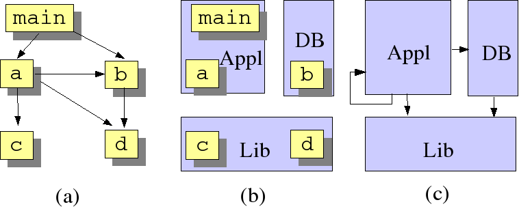
A frequently occurring problem is that we know the call relation of a system but that we want to understand it at the component level rather than at the procedure level. If it is known to which component each procedure belongs, it is possible to lift the call relation to the component level as proposed in [Kri99]. First, introduce new types to denote procedure calls as well as components of a system:
type proc = str
type comp = str
Given a calls relation
Calls2, the next step is to define the components of
the system and to define a PartOf relation between
procedures and components.
rel[proc,proc] Calls = {<"main", "a">, <"main", "b">, <"a", "b">,
                         <"a", "c">, <"a", "d">, <"b", "d">
                       }

set[comp] Components = {"Appl", "DB", "Lib"}

rel[proc, comp] PartOf = {<"main", "Appl">, <"a", "Appl">,
                          <"b", "DB">, <"c", "Lib">, <"d", "Lib">
                         }
Actual lifting, amounts to
translating each call between procedures by a call between components.
This is achieved by the following function
lift:
rel[comp,comp] lift(rel[proc,proc] aCalls, rel[proc,comp] aPartOf)=
   { <C1, C2> | <proc P1, proc P2> : aCalls,
                <comp C1, comp C2> : aPartOf[P1] x aPartOf[P2]
   }
In our example, the lifted call relation between components is obtained by
rel[comp,comp] ComponentCalls = lift(Calls2, PartOf)
and has as value:
{<"DB", "Lib">, <"Appl", "Lib">, <"Appl", "DB">, <"Appl", "Appl">}The
relevant relations for this example are shown in Figure 1.4, “(a) Calls2; (b) PartOf;
(c) ComponentCalls.”.
Now we consider the analysis of Java systems (inspired by [BNL03]. Suppose that the type class is
defined as follows
type class = str
and that the following relations are available about a Java application:
-
rel[class,class] CALL: If<is an element ofC1,C2>CALL, then some method ofC2 is called fromC1. -
rel[class,class] INHERITANCE: If<is an element ofC1,C2>INHERITANCE, then classC1 either extends classC2 orC1 implements interfaceC2. -
rel[class,class] CONTAINMENT: If <C1,C2> is an element ofCONTAINMENT, then one of the attributes of classC1 is of typeC2.
To make this more explicit, consider the class
LocatorHandle from the JHotDraw application (version
5.2) as shown here:
package CH.ifa.draw.standard;
import java.awt.Point;
import CH.ifa.draw.framework.*;
/**
* A LocatorHandle implements a Handle by delegating the
* location requests to a Locator object.
*/
public class LocatorHandle extends AbstractHandle {
private Locator fLocator;
/**
* Initializes the LocatorHandle with the given Locator.
*/
public LocatorHandle(Figure owner, Locator l) {
super(owner);
fLocator = l;
}
/**
* Locates the handle on the figure by forwarding the request
* to its figure.
*/
public Point locate() {
return fLocator.locate(owner());
}
}
It leads to the addition to the above relations of the following tuples:
-
To
CALLthe pairs<"LocatorHandle", "AbstractHandle">and<"LocatorHandle", "Locator">will be added. -
To
INHERITANCEthe pair<"LocatorHandle", "AbstractHandle">will be added. -
To
CONTAINMENTthe pair<"LocatorHandle", "Locator">will be added.
Cyclic structures in object-oriented systems makes understanding hard. Therefore it is interesting to spot classes that occur as part of a cyclic dependency. Here we determine cyclic uses of classes that include calls, inheritance and containment. This is achieved as follows:
rel[class,class] USE = CALL union CONTAINMENT union INHERITANCE
set[str] ClassesInCycle =
{C1 | <class C1, class C2> : USE+, C1 == C2}First,
we define the USE relation as the union of the three
available relations CALL,
CONTAINMENT and INHERITANCE. Next,
we consider all pairs
<C1,
C2> in the
transitive closure of the USE relation such that
C1 and
C2 are equal. Those
are precisely the cases of a class with a cyclic dependency on itself.
Probably, we do not only want to know which classes occur in a cyclic
dependency, but we also want to know which classes are involved in such
a cycle. In other words, we want to associate with each class a set of
classes that are responsible for the cyclic dependency. This can be done
as follows.
rel[class,class] USE = CALL union CONTAINMENT union INHERITANCE
set[class] CLASSES = carrier(USE)
rel[class,class] USETRANS = USE+
rel[class,set[class]] ClassCycles =
   {<C, USETRANS[C]> | class C : CLASSES, <C, C> in USETRANS }
First,
we introduce two new shorthands: CLASSES and
USETRANS. Next, we consider all classes
C with a cyclic dependency and add the pair
<C, USETRANS[C]> to the relation
ClassCycles. Note that USETRANS[C]
is the right image of the relation USETRANS for
element C, i.e., all classes that can be called
transitively from class C.
Consider the following program in the toy language Pico: (This is an extended version of the example presented earlier in [Kli03].)
[ 1] begin declare x : natural, y : natural,
[ 2]              z : natural, p : natural;
[ 3]  x := 3;
[ 4]  p := 4;
[ 5]  if q then
[ 6]        z := y + x
[ 7]  else
[ 8]        x := 4
[ 9]  fi;
[10]  y := z
[11] end
Inspection of this program learns that some of the
variables are being used before they have been initialized. The
variables in question are q (line 5),
y (line 6), and z (line 10). It is
also clear that variable p is initialized (line 4),
but is never used. How can we automate these kinds of analysis? Recall
from ??? that we follow
extract-enrich-view paradigm to approach such a problem. The first step
is to determine which elementary facts we need about the program. For
this and many other kinds of program analysis, we need at least the
following:
-
The control flow graph of the program. We represent it by a relation
PRED(for predecessor) which relates each statement with each predecessors. -
The definitions of each variable, i.e., the program statements where a value is assigned to the variable. It is represented by the relation
DEFS. -
The uses of each variable, i.e., the program statements where the value of the variable is used. It is represented by the relation
USES.
In this example, we will use line numbers to identify the statements in the program. (In the section called “Using Locations to Represent Program Fragments”, we will use locations to represent statements.) Assuming that there is a tool to extract the above information from a program text, we get the following for the above example:
type expr = int
type varname = str
expr ROOT = 1
rel[expr,expr] PRED = { <1,3>, <3,4>, <4,5>, <5,6>, <5,8>,
                        <6,10>, <8,10>
                      }
rel[expr,varname] DEFS = { <3,"x">, <4,"p">, <6,"z">,
                           <8,"x">, <10,"y">
                         }
rel[expr,varname] USES = { <5,"q">, <6,"y">, <6,"x">, <10,"z"> }
This
concludes the extraction phase. Next, we have to enrich these basic
facts to obtain the initialized variables in the program. So, when is a
variable V in some statement
S initialized? If we execute the program
(starting in ROOT), there may be several possible
execution path that can reach statement S.
All is well if all these execution path contain a
definition of V. However, if one or more of
these path do not contain a definition of
V, then V may be
uninitialized in statement S. This can be
formalized as follows:
rel[expr,varname] UNINIT =
   { <E, V> | <expr E, varname V>: USES,
              E in reachX({ROOT}, DEFS[-,V], PRED)
   }
We analyze this definition in detail:
-
<expr E, varname V> : USESenumerates all tuples in theUSESrelation. In other words, we consider the use of each variable in turn. -
E in reachX({ROOT}, DEFS[-,V], PRED)is a test that determines whether statementSis reachable from theROOTwithout encountering a definition of variableV.-
{ROOT}represents the initial set of nodes from which all path should start. -
DEFS[-,V]yields the set of all statements in which a definition of variableVoccurs. These nodes form the exclusion set forreachX: no path will be extended beyond an element in this set. -
PREDis the relation for which the reachability has to be determined. -
The result of
reachX({ROOT}, DEFS[-,V], PRED)is a set that contains all nodes that are reachable from theROOT(as well as all intermediate nodes on each path). -
Finally,
E in reachX({ROOT}, DEFS[-,V], PRED)tests whether expressionEcan be reached from theROOT.
-
-
The net effect is that
UNINITwill only contain pairs that satisfy the test just described.
When we execute the resulting Rscript (i.e., the declarations of
ROOT, PRED,
DEFS, USES and
UNINIT), we get as value for
UNINIT:
{<5, "q">, <6, "y">, <10, "z">}and this is in concordance with the informal analysis given at the beginning of this example.
As a bonus, we can also determine the unused variables in a program, i.e., variables that are defined but are used nowhere. This is done as follows:
set[var] UNUSED = range(DEFS) \ range(USES)
Taking
the range of the relations DEFS and
USES yields the variables that are defined,
respectively, used in the program. The difference of these two sets
yields the unused variables, in this case
{"p"}.
Warning
Fix the following
\begin{figure}[tb] \begin{center} \epsfig{figure=figs/meta-pico.eps,width=6cm} \hspace*{0.5cm} \epsfig{figure=figs/pico-example.eps,width=6cm} \end{center} \hrulefill \caption{\label{FIG:meta-pico}Checking undefined variables in Pico programs using the ASF+SDF Meta-Environment. On the left, main window of Meta-Environment with error messages related to Pico program shown on the right.{\bf THIS FIGURE IS OUTDATED}} \end{figure}
One aspect of the example we have just seen is artificial: where
do these line numbers come from that we used to indicate expressions in
the program? One solution is to let the extraction phase generate
locations to precisely indicate relevant places in
the program text. Recall from the section called “Elementary Types and Values”, that a location consists of a
file name, a begin line, a begin position, an end line, and an end
position. Also recall that locations can be compared: a location
A1 is smaller than
another location A2,
if A1 is textually
contained in A2. By
including locations in the final answer of a relational expression,
external tools will be able to highlight places of interest in the
source text.
The first step, is to define the type expr as
aliases for loc (instead of
int):
type expr = loc
type varname = str
Of course, the actual relations are now represented differently.
For instance, the USES relation may now look
like
{ <area-in-file("/home/paulk/example.pico",
                area(5,5,5,6,106,1)), "q">,
  <area-in-file("/home/paulk/example.pico",
                area(6,13,6,14,127,1)), "y">,
  <area-in-file("/home/paulk/example.pico",
                area(6,17,6,18,131,1)), "x">,
  <area-in-file("/home/paulk/example.pico",
                area(10,7,10,8,168,1)), "z">
}
The definition of UNINIT can be nearly reused
as is. The only thing that remains to be changed is to map the
(expression, variable-name) tuples to (variable-name,
variable-occurrence) tuples, for the benefit of the precise highlighting
of the relevant variables. We define a new type var
to represent variable occurrences and an auxiliary set that
VARNAMES that contains all variable names:
type var = loc
set[varname] VARNAMES = range(DEFS) union range(USES)
Remains the new definition of UNINIT:
rel[var, varname] UNINIT =
   { <V, VN>| var-name VN : VARNAMES,
              var V : USES[-,VN],
              expr E : reachX({ROOT}, DEFS[-,VN], PRED),
              V <= E
   }
This definition can be understood as follows:
-
var-name VN : VARNAMESgenerates all variable names. -
var V : USES[-,VN]generates all variable usesVfor variables with nameVN. -
As before,
expr E : reachX({ROOT}, DEFS[-,VN],
          PRED)
generates all expressionsEthat can be reached from the start of the program without encountering a definition for variables namedVN. -
V
<= Etests whether variable useVis enclosed in that expression (using a comparison on locations). If so, we have found an uninitialized occurrence of the variable namedVN.
Warning
Fix reference
In Figure~\ref{FIG:meta-pico} it is shown how checking of Pico programs in the ASF+SDF Meta-Environment looks like.
The cyclomatic complexity of a program is
defined as e - n +
2, where e and n
are the number of edges and nodes in the control flow graph,
respectively. It was proposed by McCabe [McC76] as a
measure of program complexity. Experiments have shown that programs with
a higher cyclomatic complexity are more difficult to understand and test
and have more errors. It is generally accepted that a program, module or
procedure with a cyclomatic complexity larger than 15 is too
complex. Essentially, cyclomatic complexity measures the
number of decision points in a program and can be computed by counting
all if statement, case branches in switch statements and the number of
conditional loops. Given a control flow in the form of a predecessor
relation rel[stat,stat] PRED between statements, the
cyclomatic complexity can be computed in an Rscript as follows:
int cyclomatic-complexity(rel[stat,stat] PRED) =
    #PRED - #carrier(PRED) + 2
The number of edges
e is equal to the number of tuples in
PRED. The number of nodes
n is equal to the number of elements in the
carrier of PRED, i.e., all elements that occur in a tuple in
PRED.
Dataflow analysis is a program analysis technique that forms the basis for many compiler optimizations. It is described in any text book on compiler construction, e.g. [ASU86]. The goal of dataflow analysis is to determine the effect of statements on their surroundings. Typical examples are:
-
Dominators (the section called “Dominators”): which nodes in the flow dominate the execution of other nodes?
-
Reaching definitions (the section called “Reaching Definitions”): which definitions of variables are still valid at each statement?
-
Live variables (the section called “Live Variables”): of which variables will the values be used by successors of a statement?
-
Available expressions: an expression is available if it is computed along each path from the start of the program to the current statement.
A node d of a flow graph
dominates a node n, if
every path from the initial node of the flow graph to
n goes through d
[ASU86] (Section 10.4). Dominators play a
role in the analysis of conditional statements and loops. The function
dominators that computes the dominators for a given
flow graph PRED and an entry node
ROOT is defined as follows:
rel[stat,stat] dominators(rel[stat,stat] PRED, int ROOT) =
   DOMINATES
where
    set[int] VERTICES = carrier(PRED)

    rel[int,set[int]] DOMINATES =
    { <V,  VERTICES \ {V, ROOT} \ reachX({ROOT}, {V}, PRED)> |
      int V : VERTICES }
endwhere
First, the auxiliary set VERTICES (all the
statements) is computed. The relation DOMINATES
consists of all pairs <
such thatS,
{S1,...,Sn}>
-
Siis not an initial node or equal toS. -
Sicannot be reached from the initial node without going throughS.
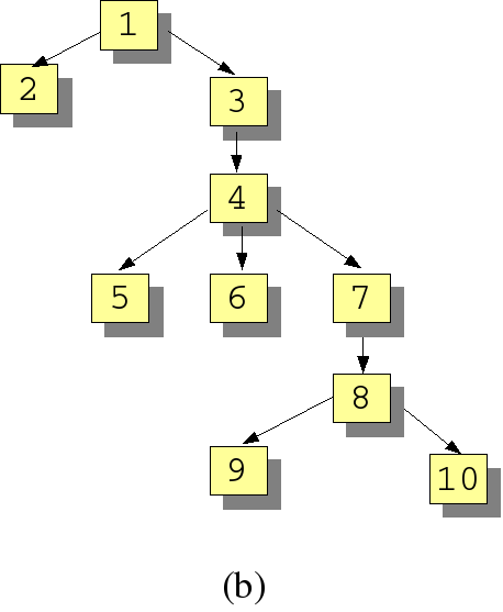
Consider the flow graph
rel[int,int] PRED = {
<1,2>, <1,3>,
<2,3>,
<3,4>,
<4,3>,<4,5>, <4,6>,
<5,7>,
<6,7>,
<7,4>,<7,8>,
<8,9>,<8,10>,<8,3>,
<9,1>,
<10,7>
}
It is illustrated inFigure 1.5, “Flow graph”
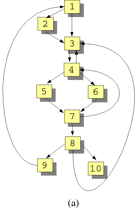
The result of applying dominators to it
is as follows:
{<1, {2, 3, 4, 5, 6, 7, 8, 9, 10}>,
<2, {}>,
<3, {4, 5, 6, 7, 8, 9, 10}>,
<4, {5, 6, 7, 8, 9, 10}>,
<5, {}>,
<6, {}>,
<7, {8, 9, 10}>,
<8, {9, 10}>,
<9, {}>,
<10, {}>}
The resulting dominator
tree is shown in Figure 1.6, “Dominator tree”.
The dominator tree has the initial node as root and each node
d in the tree only dominates its
descendants in the tree.
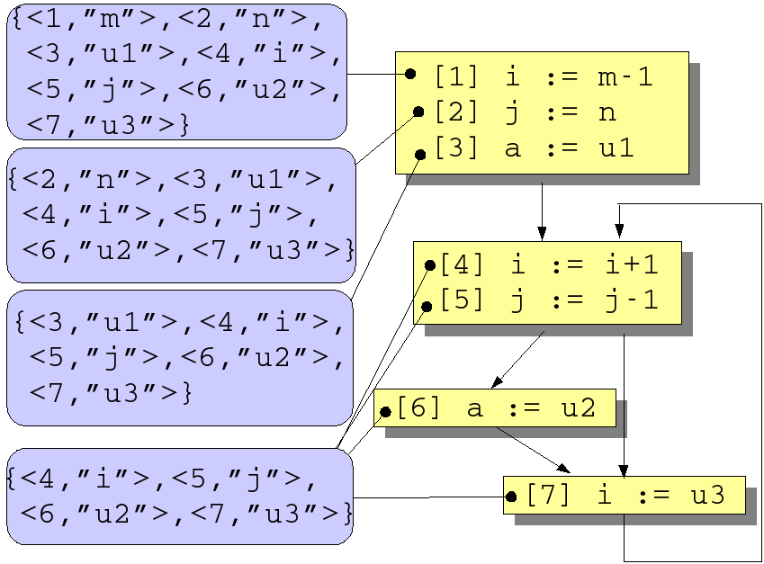
We illustrate the calculation of reaching definitions using the example in Figure 1.7, “Flow graph for various dataflow problems” which was inspired by [ASU86] (Example 10.15).
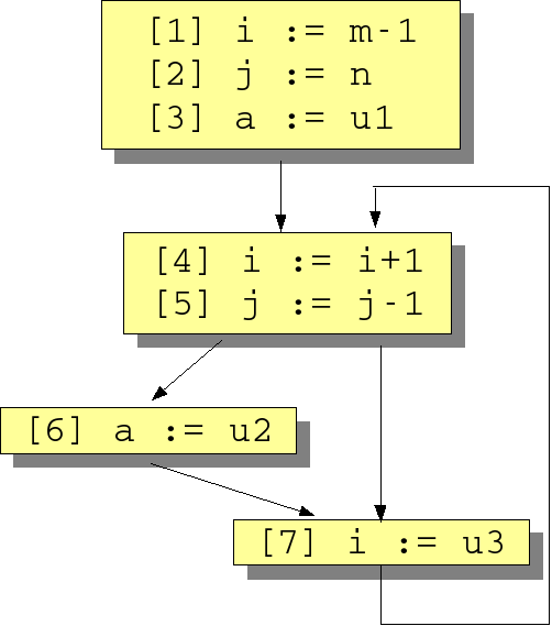
As before, we assume the following basic relations
PRED, DEFS and
USES about the program:
type stat = int
type var = str
rel[stat,stat] PRED = { <1,2>, <2,3>, <3,4>, <4,5>, <5,6>,
                        <5,7>, <6,7>, <7,4>
                      }
rel[stat, var] DEFS = { <1, "i">, <2, "j">, <3, "a">, <4, "i">,
                       <5, "j">, <6, "a">, <7, "i">
                      }
rel[stat, var] USES = { <1, "m">, <2, "n">, <3, "u1">, <4, "i">,
                        <5, "j">, <6, "u2">, <7, "u3">
                      }
For convenience, we introduce a notion def
that describes that a certain statement defines some variable and we
revamp the basic relations into a more convenient format using this
new type:
type def  = <stat theStat, var theVar>

rel[stat, def] DEF = {<S, <S, V>> | <stat S, var V> : DEFS}
rel[stat, def] USE = {<S, <S, V>> | <stat S, var V> : USES}
The
new DEF relation gets as value:
{ <1, <1, "i">>, <2, <2, "j">>, <3, <3, "a">>, <4, <4, "i">>,
  <5, <5, "j">>, <6, <6, "a">>, <7, <7, "i">>
}
and USE gets as value:
{ <1, <1, "m">>, <2, <2, "n">>, <3, <3, "u1">>, <4, <4, "i">>,
  <5, <5, "j">>, <6, <6, "u2">>, <7, <7, "u3">>
}
Now we are ready to define an important new relation
KILL. KILL defines which
variable definitions are undone (killed) at each statement and is
defined as follows:
rel[stat, def] KILL =
   {<S1, <S2, V>> | <stat S1, var V> : DEFS,
                    <stat S2, V> : DEFS,
                    S1 != S2
   }
In this definition, all variable definitions are compared
with each other, and for each variable definition all
other definitions of the same variable are placed
in its kill set. In the example, KILL gets the
value
{ <1, <4, "i">>, <1, <7, "i">>, <2, <5, "j">>, <3, <6, "a">>,
  <4, <1, "i">>, <4, <7, "i">>, <5, <2, "j">>, <6, <3, "a">>,
  <7, <1, "i">>, <7, <4, "i">>
}
and, for instance, the definition of variable
i in statement 1 kills the
definitions of i in statements 4
and 7. Next, we introduce the collection of
statements
set[stat] STATEMENTS = carrier(PRED)
which
gets as value {1, 2, 3, 4, 5, 6, 7} and two
convenience functions to obtain the predecessor, respectively, the
successor of a statement:
set[stat] predecessor(stat S) = PRED[-,S]
set[stat] successor(stat S) = PRED[S,-]
After these preparations, we are ready to formulate the reaching
definitions problem in terms of two relations IN
and OUT. IN captures all the
variable definitions that are valid at the entry of each statement and
OUT captures the definitions that are still valid
after execution of each statement. Intuitively, for each statement
S, IN[S] is equal to the union
of the OUT of all the predecessors of
S. OUT[S], on the other hand, is
equal to the definitions generated by S to which we
add IN[S] minus the definitions that are killed in
S. Mathematically, the following set of equations
captures this idea for each statement:
Warning
Fix expression
[ IN[S] = \bigcup_{P \in predecessor of S} OUT[P] \]
\[ OUT[S] = DEF[S] \cup (IN[S] - KILL[S]) \]
This idea can be expressed in Rscript quite literally:
equations
  initial
        rel[stat,def] IN init {}
        rel[stat,def] OUT init DEF
  satisfy
        IN  = {<S, D> | stat S : STATEMENTS,
                        stat P : predecessor(S),
                        def D : OUT[P]}
        OUT = {<S, D> | stat S : STATEMENTS,
                        def D : DEF[S] union (IN[S] \ KILL[S])}
end equations
First, the relations IN and
OUT are declared and initialized. Next, two
equations are given that very much resemble the ones given
above.
Figure 1.8. Reaching definitions for flow graph in Figure 1.7, “Flow graph for various dataflow problems”
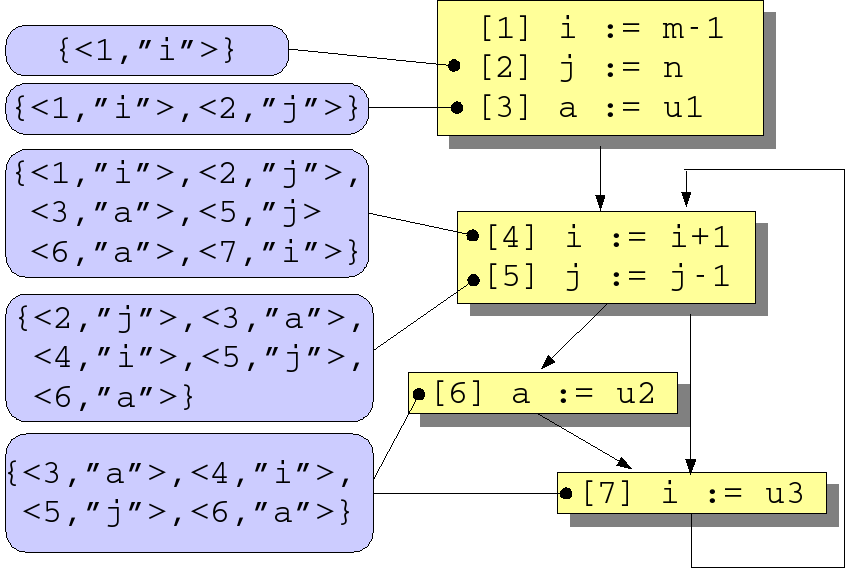
For our running example (Figure 1.8, “Reaching definitions for flow graph in Figure 1.7, “Flow graph for various dataflow problems””) the results are as follows
(see Figure 1.8, “Reaching definitions for flow graph in Figure 1.7, “Flow graph for various dataflow problems””). Relation
IN has as value:
{ <2, <1, "i">>, <3, <2, "j">>, <3, <1, "i">>, <4, <3, "a">>,
  <4, <2, "j">>, <4, <1, "i">>, <4, <7, "i">>, <4, <5, "j">>,
  <4, <6, "a">>, <5, <4, "i">>, <5, <3, "a">>, <5, <2, "j">>,
  <5, <5, "j">>, <5, <6, "a">>, <6, <5, "j">>, <6, <4, "i">>,
  <6, <3, "a">>, <6, <6, "a">>, <7, <5, "j">>, <7, <4, "i">>,
  <7, <3, "a">>, <7, <6, "a">>
}
If we consider statement 3, then the
definitions of variables i and j
from the preceding two statements are still valid. A more interesting
case are the definitions that can reach statement
4:
-
The definitions of variables
a,jandifrom, respectively, statements3,2and1. -
The definition of variable
ifrom statement7(via the backward control flow path from7to4). -
The definition of variable
jfrom statement5(via the path5,7,4). -
The definition of variable
afrom statement6(via the path6,7,4).
Relation OUT has as value:
{ <1, <1, "i">>, <2, <2, "j">>, <2, <1, "i">>, <3, <3, "a">>,
  <3, <2, "j">>, <3, <1, "i">>, <4, <4, "i">>, <4, <3, "a">>,
  <4, <2, "j">>, <4, <5, "j">>, <4, <6, "a">>, <5, <5, "j">>,
  <5, <4, "i">>, <5, <3, "a">>, <5, <6, "a">>, <6, <6, "a">>,
  <6, <5, "j">>, <6, <4, "i">>, <7, <7, "i">>, <7, <5, "j">>,
  <7, <3, "a">>, <7, <6, "a">>
}
Observe, again for statement 4, that all
definitions of variable i are missing in
OUT[4] since they are killed by the definition of
i in statement 4 itself.
Definitions for a and j are,
however, contained in OUT[4]. The result of
reaching definitions computation is illustrated in Figure 1.8, “Reaching definitions for flow graph in Figure 1.7, “Flow graph for various dataflow problems””. The above definitions are
used to formulate the function
reaching-definitions. It assumes appropriate
definitions for the types stat and
var. It also assumes more general versions of
predecessor and successor. We
will use it later on in the section called “Program Slicing”
when defining program slicing. Here is the definition of
reaching-definitions:
type def  = <stat theStat, var theVar>
type use  = <stat theStat, var theVar>

set[stat] predecessor(rel[stat,stat] P, stat S) = P[-,S]

set[stat] successor(rel[stat,stat] P, stat S) = P[S,-]

rel[stat, def] reaching-definitions(rel[stat,var] DEFS,
                                    rel[stat,stat] PRED) =
   IN
where
    set[stat] STATEMENT = carrier(PRED)

    rel[stat,def] DEF  = {<S,<S,V>> | <stat S, var V> : DEFS}

    rel[stat,def] KILL =
        {<S1, <S2, V>> | <stat S1, var V> : DEFS,
                         <stat S2, V> : DEFS,
                         S1 != S2
        }

    equations
       initial
           rel[stat,def] IN init {}
           rel[stat,def] OUT init DEF
       satisfy
           IN  =  {<S, D> | int S : STATEMENT,
                            stat P : predecessor(PRED,S),
                            def D : OUT[P]}
           OUT = {<S, D> |  int S : STATEMENT,
                            def D : DEF[S] union (IN[S] \ KILL[S])}
    end equations
end where
The live variables of a statement are those variables whose value will be used by the current statement or some successor of it. The mathematical formulation of this problem is as follows:
Warning
Fix expression
\[ IN[S] =USE[S] \cup (OUT[S] - DEF[S]) \]
\[ OUT[S] = \bigcup_{S' \in successor of S} IN[S'] \]
The first equation says that a variable is live coming into a statement if either it is used before redefinition in that statement or it is live coming out of the statement and is not redefined in it. The second equation says that a variable is live coming out of a statement if and only if it is live coming into one of its successors.
This can be expressed in Rscript as follows:
equations
  initial
      rel[stat,def] LIN init {}
      rel[stat,def] LOUT init DEF
  satisfy
      LIN = { < S, D> | stat S : STATEMENTS,
                        def D : USE[S] union (LOUT[S] \ (DEF[S]))
            }
      LOUT= { < S, D> | stat S : STATEMENTS,
                        stat Succ : successor(S),
                        def D : LIN[Succ]
            }
end equations
The results of live variable analysis for our running example are illustrated in Figure 1.9, “Live variables for flow graph in Figure 1.7, “Flow graph for various dataflow problems””.
Program slicing is a technique proposed by Weiser [Wei84] for automatically decomposing programs in parts by analyzing their data flow and control flow. Typically, a given statement in a program is selected as the slicing criterion and the original program is reduced to an independent subprogram, called a slice, that is guaranteed to represent faithfully the behavior of the original program at the slicing criterion. An example will illustrate this:
[ 1] read(n)            [ 1] read(n)           [ 1] read(n)
[ 2] i := 1             [ 2] i := 1            [ 2] i := 1
[ 3] sum := 0           [ 3] sum := 0
[ 4] product := 1                              [ 4] product := 1
[ 5] while i<= n do     [ 5] while i<= n do    [ 5] while i<= n do
     begin                   begin                  begin
[ 6]   sum := sum + i   [ 6]   sum := sum + i
[ 7]   product :=                              [ 7]   product :=
         product * i                                    product * i
[ 8]   i := i + 1       [ 8]  i := i + 1       [ 8]   i := i + 1
     end                     end                    end
[ 9] write(sum)         [ 9] write(sum)
[10] write(product)                            [10] write(product)

(a) Sample program      (b) Slice for          (c) Slice for
                           statement [9]           statement [10]
The initial program is given as (a). The slice with statement [9]
as slicing criterion is shown in (b): statements [4]
and [7] are irrelevant for computing statement
[9] and do not occur in the slice. Similarly, (c)
shows the slice with statement [10] as slicing
criterion. This particular form of slicing is called backward
slicing. Slicing can be used for debugging and program
understanding, optimization and more. An overview of slicing techniques
and applications can be found in [Tip95]. Here we will
explore a relational formulation of slicing adapted from a proposal in
[JR94]J. The basic ingredients of the
approach are as follows:
-
We assume the relations
PRED,DEFSandUSESas before. -
We assume an additional set
CONTROL-STATEMENTthat defines which statements are control statements. -
To tie together dataflow and control flow, three auxiliary variables are introduced:
-
The variable
TESTrepresents the outcome of a specific test of a conditional statement. The conditional statement definesTESTand all statements that are control dependent on this conditional statement will useTEST. -
The variable
EXECrepresents the potential execution dependence of a statement on some conditional statement. The dependent statement definesEXECand an explicit (control) dependence is made betweenEXECand the correspondingTEST. -
The variable
CONSTrepresents an arbitrary constant.
-
The calculation of a (backward) slice now proceeds in six steps:
-
Compute the relation
rel[use,def] use-defthat relates all uses to their corresponding definitions. The functionreaching-definitionsas shown earlier in the section called “Reaching Definitions”does most of the work. -
Compute the relation
rel[def,use]
          def-use-per-stat
that relates the internal definitions and uses of a statement. -
Compute the relation
rel[def,use]
          control-dependence
that links allEXECs to the correspondingTESTs. -
Compute the relation
rel[use,def]
          use-control-def
combines use/def dependencies with control dependencies. -
After these preparations, compute the relation
rel[use,use] USE-USEthat contains dependencies of uses on uses. -
The backward slice for a given slicing criterion (a use) is now simply the projection of
USE-USEfor the slicing criterion.
This informal description of backward slicing can now be expressed in Rscript:
set[use] BackwardSlice(
    set[stat] CONTROL-STATEMENT,
    rel[stat,stat] PRED,
    rel[stat,var] USES,
    rel[stat,var] DEFS,
    use Criterion)
= USE-USE[Criterion]

where
    rel[stat, def] REACH = reaching-definitions(DEFS, PRED)

    rel[use,def] use-def =
       { <<S1,V>, <S2,V>> | <stat S1, var V> : USES,
                            <stat S2, V> : REACH[S1]
       }

    rel[def,use] def-use-per-stat  =
       {<<S,V1>, <S,V2>> | <stat S, var V1> : DEFS,
                           <S, var V2> : USES
       }
             union
       {<<S,V>, <S,"EXEC">> | <stat S, var V> : DEFS}
             union
       {<<S,"TEST">,<S,V>> | stat S : CONTROL-STATEMENT,
                             <S, var V> : domainR(USES, {S})
       }

    rel[stat, stat] CONTROL-DOMINATOR =
       domainR(dominators(PRED), CONTROL-STATEMENT)

    rel[def,use] control-dependence  =
       { <<S2, "EXEC">,<S1,"TEST">> |
         <stat S1, stat S2> : CONTROL-DOMINATOR
       }

    rel[use,def] use-control-def = use-def union control-dependence

    rel[use,use] USE-USE = (use-control-def o def-use-per-stat)*

endwhere
Let's apply this to the example from the start of this section and assume the following:
rel[stat,stat] PRED = { <1,2>, <2,3>, <3,4>, <4,5>, <5,6>, <5,9>,
                        <6,7>, <7,8>,<8,5>, <8,9>, <9,10>
                      }

rel[stat,var] DEFS  = { <1, "n">, <2, "i">, <3, "sum">,
                        <4,"product">, <6, "sum">, <7, "product">,
                        <8, "i">
                      }

rel[stat,var] USES  = { <5, "i">, <5, "n">, <6, "sum">, <6,"i">,
                        <7, "product">, <7, "i">, <8, "i">,
                        <9, "sum">, <10, "product">
                      }

set[int] CONTROL-STATEMENT = { 5 }
The result of the slice
BackwardSlice(CONTROL-STATEMENT, PRED, USES, DEFS, <9, "sum">)
will then be
 { <1, "EXEC">, <2, "EXEC">,  <3, "EXEC">, <5, "i">, <5, "n">,
   <6, "sum">, <6, "i">, <6, "EXEC">, <8, "i">, <8, "EXEC">,
   <9, "sum"> }
Take the domain of this result and we get exactly the statements in (b) of the example.
In this tutorial we have, so far, concentrated on querying and enriching facts that have been extracted from source code. As we have seen from the examples, once these facts are available, a concise Rscript suffices to do the required processing. But how is fact extraction achieved and how difficult is it? To answer these questions we first describe the workflow of the fact extraction process (the section called “Workflow for Fact Extraction”) and give strategies for fact extraction (the section called “Strategies for Fact Extraction”).
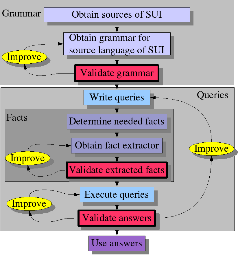
Figure 1.10, “Workflow for fact extraction” shows a typical workflow for fact extraction for a System Under Investigation (SUI). It assumes that the SUI uses only one programming language and that you need only one grammar. In realistic cases, however, several such grammars may be needed. The workflow consists of three main phases:
-
Grammar: Obtain and improve the grammar for the source language of the SUI.
-
Facts: Obtain and improve facts extracted from the SUI.
-
Queries: Write and improve queries that give the desired answers.
Of course, it may happen that you have a lucky day and that extracted facts are readily available or that you can reuse a good quality fact extractor that you can apply to the SUI. On ordinary days you have the above workflow as fall-back. It may come as a surprise that there is such a strong emphasis on validation in this workflow. The reason is that the SUI is usually a huge system that defeats manual inspection. Therefore we must be very careful that we validate the outcome of each phase.
Grammar. In many cases there is no canned grammar available that can be used to parse the programming language dialect used in the SUI. Usually an existing grammar can be adjusted to that dialect, but then it is then mandatory to validate that the adjusted grammar can be used to parse the sources of the SUI.
Facts. It may happen that the facts extracted from the source code are wrong. Typical error classes are:
-
Extracted facts are wrong: the extracted facts incorrectly state that procedure
Pcalls procedureQbut this is contradicted by a source code inspection. -
Extracted facts are incomplete: the inheritance between certain classes in Java code is missing.
The strategy to validate extracted facts differ per case but here are three strategies:
-
Postprocess the extracted facts (using Rscript, of course) to obtain trivial facts about the source code such as total lines of source code and number of procedures, classes, interfaces and the like. Next validate these trivial facts with tools like
wc(word and line count),grep(regular expression matching) and others. -
Do a manual fact extraction on a small subset of the code and compare this with the automatically extracted facts.
-
Use another tool on the same source and compare results whenever possible. A typical example is a comparison of a call relation extracted with different tools.
Queries. For the validation of the answers to the queries essentially the same approach can be used as for validating the facts. Manual checking of answers on random samples of the SUI may be mandatory. It also happens frequently that answers inspire new queries that lead to new answers, and so on.
The following global scenario's are available when writing a fact extractor:
-
Dump-and-Merge: Parse each source file, extract the relevant facts, and return the resulting (partial) Rstore. In a separate phase, merge all the partial Rstores into a complete Rstore for the whole SUI. The tool {\tt merge-rstores} is available for this.
-
Extract-and-Update: Parse each source file, extract the relevant facts, and add these directly to the partial Rstore that has been constructed for previous source files.
The experience is that the Extract-and-Update is more efficient. A second consideration is the scenario used for the fact extraction per file. Here there are again two possibilities:
-
All-in-One: Write one function that extracts all facts in one traversal of the source file. Typically, this function has an Rstore as argument and returns an Rstore as well. During the visit of specific language constructs additions are made to named sets or relations in the Rstore.
-
Separation-of-Concerns: Write a separate function for each fact you want to extract. Typically, each function takes a set or relation as argument and returns an updated version of it. At the top level all these functions are called and their results are put into an Rstore. This strategy is illustrated in Figure 1.11, “Separation-of-Concerns strategy for fact extraction”.
The experience here is that everybody starts with the All-in-One strategy but that the complexities of the interactions between the various fact extraction concerns soon start to hurt. The advice is therefore to use the Separation-of-Concerns strategy even if it may be seem to be less efficient since it requires a traversal of the source program for each extracted set or relation.
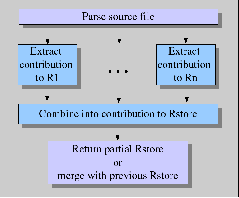
Although facts can be extracted in many ways, ASF+SDF is the tool of preference to do this. Examples are given In XXX.
Warning
Fix reference
It is not unusual that the effort that is needed to write a fact extractor is much larger than the few lines of Rscript that are sufficient for the further processing of these facts. What can we learn from this observation? First, that even in simple cases fact extraction is more complicated than the processing of these facts. This may be due to the following:
-
The facts we are interested in may be scattered over different language constructs. This implies that the fact extractor has to cover all these cases.
-
The extracted facts are completely optimized for relational processing but places a burden on the fact extractor to perform this optimization.
Second, that several research questions remain unanswered:
-
Is it possible to solve (parts of) the fact extraction in a language-parametric way. In other words, is it possible to define generic extraction methods that apply to multiple languages?
-
Is a further integration of fact extraction with relational processing desirable? Is it, for instance, useful to bring some of the syntactic program domains like expressions and statements to the relational domain?
Table 1.10. Table of Built-in Operators
Table 1.11. Table of Built-in Functions
[BNL03] Simple and efficient relational querying of software structures. Proceedings of the 10th IEEE Working Conference on Reverse Engineering (WCRE 2003). . 2003. To appear.
[KN96] Drawing graphs with dot. Technical report. AT&T Bell Laboratories. Murray Hill, NJ. 1996. See also www.graphviz.org.
[FKO98] A relational approach to support software architecture analysis. 371--400. Software Practice and Experience. 4. april 1998.
[Hol96] Binary relational algebra applied to software architecture. CSRI345. University of Toronto. march 1996.
[JR94] A new model of program dependences for reverse engineering. 2--10. Proceedings of the 2nd ACM SIGSOFT symposium on Foundations of software engineering. . ACM SIGSOFT Software Engineering Notes. <seriesvolnum>19</seriesvolnum>1994.
[Kli03] How understanding and restructuring differ from compiling---a rewriting perspective. 2--12. Proceedings of the 11th International Workshop on Program Comprehension (IWPC03). . 2003. IEEE Computer Society.
[MK88] Rigi -- a system for programming-in-the-large.. 80--86,. Proceedings of the 10th International Conference on Software Engineering (ICSE 10),. . April 1988.