Table of Contents
- Introduction
- Preparations
- The toy language Pico
- Define the syntax for Pico
- Define a typechecker for Pico
- Defining an evaluator for Pico
- Defining a compiler for Pico
- Intermezzo: traversal functions
- Simple trees
- Counting tree nodes (classical solution)
- Counting tree nodes (using an accumulator)
- Increment and modify tree leaves (using a transformer)
- Increment with variable amount and modify tree leaves (using transformer)
- Tree replacement
- A real example: COBOL transformation
- A funny Pico typechecker
- Take home points
- Define a fact extractor for Pico
- To Do
Warning
This document is work in progress. See ToDo section.
You are interested in using ASF+SDF to define various aspects of a programming language or domain-specific language but you do now want to wade through all the details in the manual (The Language Specification Formalism ASF+SDF)? In that case, this article may be for you. We take the toy language Pico as starting point and walk you through its syntax, typechecking, formatting, execution and more. We do this while assuming zero knowledge of ASF+SDF or The ASF+SDF Meta-Environment.
ASF+SDF can be used to define various aspects of programming langauges and The ASF+SDF Meta-Environment can be used to edit and run these specifications.
The goal of ASF+SDF is to define the syntax (form) and semantics (meaning) of programming languages and domain-specific languages. The Syntax Definition Formalism (SDF) is used to define syntactic aspects including:
-
Lexical syntax (keywords, comments, string constants, whiete space, ...).
-
Context-free syntax (declarations, statements, ...).
The Algebraic Specification Formalism (ASF) is used to define semantic aspects such as:
-
Type checking (are the variables that are used declared and are they used in a type-correct way?).
-
Formatting (display the original program using user-defined rules for indentation and formatting).
-
Fact extraction (extract all procedure calls or all declarations and uses of variables).
-
Execution (run the program with given input values).
By convention, all these language aspects are located in dedicated subdirectories of a language definition:
-
syntax(definitions for the syntax). -
check(definitions for type checking). -
format(definitions for formatting). -
extract(definitions for fact extraction). -
run(definitions for running a program). -
debug(definitions for debugging a program).
Apart from giving a standard structure to all language definitions, this organization also enables the seamless integration of these aspects in the user-interface of The Meta-Environment.
The goal of The ASF+SDF Meta-Environment (or The Meta-Environment for short) is to provide an Interactive Development Environment for ASF+SDF specifications. It supports interactive editing, checking and execution of ASF+SDF specifications. Behind the scenes, this implies the following tasks:
-
Providing a graphical user-interface with editors and various visualization tools.
-
Tracking changes to specification modules.
-
Parsing and checking specification modules.
-
Generating parsers for the syntax modules (SDF) that have been changed.
-
Generating rewriter engines for the equations modules (ASF) that have been changed.
-
Applying the ASF+SDF specification to programs in the language that is being defined by that specification.
The intended user experience of The Meta-Environment is the seamless automation of all these tasks.
This article guides you through the various stages of writing
language definitions in ASF+SDF. The following documents (all available
at http://www.meta-environment.org) will help you to learn
more:
-
The basic concepts of syntax analysis are given in the article "Syntax Analysis".
-
The basic concepts of term rewriting are discussed in the article "Term Rewriting".
-
"The Syntax Definition Formalism SDF" is the reference manual for the SDF formalism.
-
"The Language Specification Formalism ASF+SDF" is the reference manual for the ASF+SDF formalism.
-
"Guided tour: Playing with Booleans" is a flash movie that gives you a quick overview of the user-interface of the Meta-Environment.
The anatomies of a complete ASF+SDF specification as well as that of a single module are needed to understand any language definition.
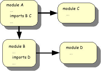
An ASF+SDF specification consists of a collection of modules as
shown in the following Figure 1.1, “Module structure of an ASF+SDF specification”. A module can
import other modules and this can be understood as the textual inclusion
of the imported modules. In this example, the text of modules
B, C and D is
literally inserted in module A.
A single module has the following structure:
moduleModuleName
ImportSection*
ExportOrHiddenSection*equations
ConditionalEquation*
Notes:
| |
The name of this module. It may be followed by parameters. |
| |
Zero or more sections that describe modules to be imported by this module. |
| |
The grammar elements (such as |
 |
The equations of the module that define the meaning of the grammar elements. Equations come in two flavours. Unconditional: [<TagId>] <Term1> = <Term2> and conditional: [<TagId>] <Condition1>, <Condition2>, ... =============================== <Term1> = <Term2> In the unconditional case, an attempt is made to match Term1 and if this succeeds it is replaced by Term2 (after proper replacement of variables that result from the match). In the conditional case, an attempt is made to match Term1 and if this succeeds the conditions are evaluated. If all conditions are true, Term1 is replaced by Term2 (again after proper replacement of variables that may in this case result both from the match and from the evaluation of the conditions.). |
The Meta-Environment comes with a considerable library of built-in
languages and datatypes. We explore here the datatype
basic/Booleans in the ASF+SDF library.
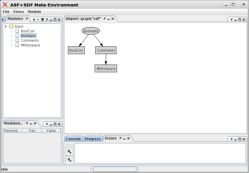
The module structure of basic/Booleans is
shown in Figure 1.2, “Modular structure of
basic/Booleans”.
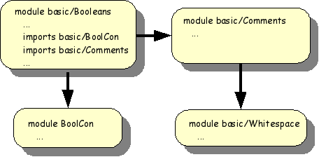
We will now discuss all these modules in turn.
Let' start with the Boolean constants:
module basic/BoolCon exports sorts BoolCon
Notes:
| |
The sort of Boolean constants is defined as
|
| |
The constants |
| |
We add a start symbol (i.e., the syntactic notion from with
all strings in this language are derived) for
|
The module Whitespace defines what the spaces and newline are:
module basic/Whitespace
exports
lexical syntax
[\ \t\n\r] -> LAYOUT {cons("whitespace")}
context-free restrictions
LAYOUT? -/- [\ \t\n\r]
Notes:
| |
A regular expression that defines space ( |
| |
Lexical syntax tends to become highly ambiguous, e.g., are
two spaces one layout symbol or two consecutive ones? Context-free
restrictions impose restrictions that resolve this. Here, optional
layout ( |
The comment conventions are defined as follows:
module basic/Comments
imports
basic/Whitespace
exports
lexical syntax
"%%" line:~[\n]* "\n" -> LAYOUT
{cons("line"),
category("Comment")}
"%" content:~[\%\n]+ "%" -> LAYOUT
{cons("nested"),
category("Comment")}
context-free restrictions
LAYOUT? -/- [\%]
Notes:
| |
Defines a line-based comment that starts with
|
| |
Define a comment that is contained within a single line
between |
| |
Again a follow restriction that forces layout followed by a comment to be included in that comment. |
After these preparations, we can now discuss the syntax part of
basic/Booleans:
module basic/Booleans imports basic/BoolCon"(" Boolean ")" -> Boolean {bracket, cons("bracket")}
context-free priorities Boolean "&" Boolean -> Boolean >
Boolean "|" Boolean -> Boolean hiddens context-free start-symbols Boolean
imports basic/Comments
variables "Bool" [0-9]* -> Boolean
Notes:
| |
Import the Boolean constants |
| |
The sort |
| |
Each Boolean constant is also a Boolean expression. This is called an injection rule or a chain rule. |
| |
The infix operators for Boolean or ( |
| |
The prefix operator |
| |
The parentheses |
| |
|
| |
Define a (hidden) start symbol for Boolean expressions. |
| |
Import |
 |
Declares Boolean variables like |
Having covered all syntactic aspects of the Booleans, we can now turn our attention to the equations:
equations [B1] true | Bool = true
Notes:
| |
Meaning of the |
| |
Meaning of |
| |
Meaning of |
The syntax of ASF+SDF equations is not fixed but depends on the syntax rules. This can be seen by making the fixed ASF+SDF syntax bold and the syntax specific for Booleans italic:
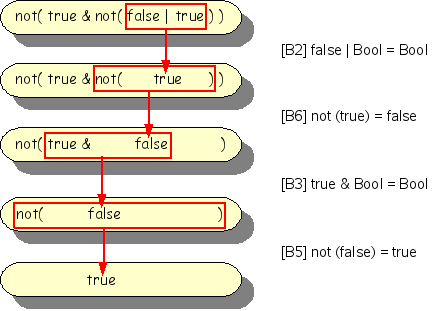
equations [B1] true | Bool = true [B2] false | Bool = Bool [B3] true & Bool = Bool [B4] false & Bool = false [B5] not ( false ) = true [B6] not ( true ) = false
This mixture of syntaxes will become even more apparent when we discuss the Pico definitions later.
The Boolean term not(true & not(false |
true)) should reduce to true (check this
for yourself before looking at Figure 1.3, “Reducing a Boolean term.”).
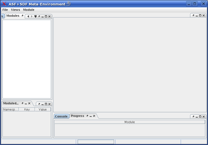
The flash movie "Guided tour: Playing with Booleans" gives you a quick overview of the user-interface of The Meta-Environment. Here we give you only some quick hints to get started. After installation, the The Meta-Environment is available as the command: asfsdf-meta. Typing this command results in the screen shown in Figure 1.4, “Initial screen of The Meta-Environment”.
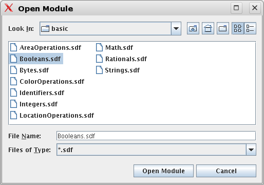
Opening the module basic/Booleans is achieved
as follows:
-
Press the menu and select the button .
-
An Open Module dialog appears that asks for the directory to Look in.
-
Select the entry ASF+SDF library and a list of choices appears.
-
Select the subdirectory
basicand selectBooleans.sdfin the list of modules that is provided. The progress so far, is shown in Figure 1.5, “Selectingbasic/Booleans.sdf”. -
Now pushing the button will open
basic/Booleansand all its imported modules. The result is shown in Figure 1.6, “After openingbasic/Booleans”.
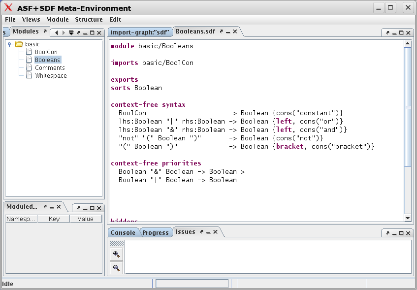
Now that the Booleans have been opened, you may want to inspect their definition yourself. There are two ways to achieve this:
-
Right click (= click with the right-most mouse button) on
Booleansin the Modules pane on the left, or -
Right click on the oval labelled
Booleansin the Import Graph pane on the right.
In both cases, a hierarchical pop-up menu will appear:
-
Select the menu entry . A new pop-up menu will appear.
-
Select the menu entry , and the syntax part of module Booleans will appear in an editor pane. The result is shown in Figure 1.7, “Opening the syntax of module Booleans”.
After these initial steps, viewing the equations and opening and reducing a Boolean term will require similar interactions with The Meta-Environment.
Important
There is no substitute for trying this out yourself.
The example of the Booleans illustrates the following points that are also valid for more complex examples:
-
Each module defines a language: in this case the language of Booleans. In other contexts one can also speak about the datatype of the Booleans. We will use language and datatype as synonyms. Other examples of languages are integers, stacks, C, and Java. We treat them all in a uniform fashion.
-
We can use the language definition for Booleans (and by implication for any language) to:
-
Create a syntax-directed editor for the Boolean language and create Boolean terms. In the context of, for instance, Java, it would be more common to say: create a syntax-directed editor for Java and create Java programs.
-
Apply the equations to this term and reduce it to a normal form (= a term that is not further reducible).
-
Import it in another module; this makes the Boolean language available for the importing module.
-
The toy language Pico has a single purpose in life: being so simple that specifications of every possible language aspect are so simple that they fit on a few pages. It can be summarized as follows:
-
There are two types: natural numbers and strings.
-
Variables have to be declared.
-
Statements are assignment, if-then-else and while-do.
-
Expressions may contain naturals, strings, variables, addition (
+), subtraction (-) and concatenation (||). -
The operators
+and-have operands of type natural and their result is natural. -
The operator
||has operands of type string and its results is also of type string. -
Tests in if-then-else statement and while-statement should be of type natural.
Let's look at a simple Pico program that computes the factorial function:
begin declare input : natural,
Notes:
| |
Pico programs do not have input/output statements, so we use variables for that purpose. |
| |
Pico has no multiplication operator so we have to simulate it with repeated addition (yes, simplicity comes at a price!). |
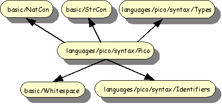
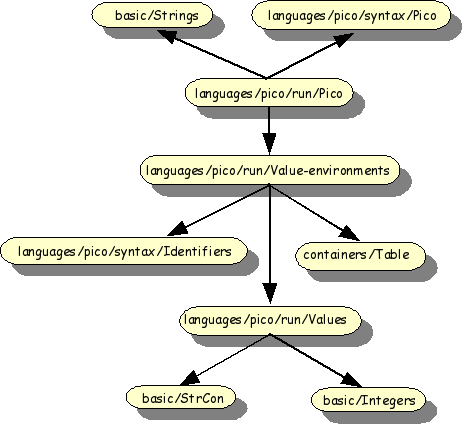
The import structure of the syntax definition of Pico is shown in
Figure 1.8, “Import structure of Pico syntax”. The modules
basic/NatCon, basic/StrCon and
basic/Whitespace are reused from the ASF+SDF library.
The modules languages/pico/syntax/Identifiers,
languages/pico/syntax/Types and
languages/pico/syntax/Pico are specified for Pico and
are now discussed in more detail.
Variables can be declared in Pico programs with one of two types: "natural number" or "string". This is defined as follows:
module languages/pico/syntax/Types exports sorts TYPE
Notes:
| |
|
| |
The constants |
| |
The constant |
Identifiers are used for the names of variables in Pico programs. They are defined as follows:
module languages/pico/syntax/Identifiers exports sorts PICO-ID
Notes:
| |
|
| |
The overall effect of this definition is that Pico identifiers start with a lower case letter that can be followed by lower case letters or by digits. |
| |
Defines the longest match for Pico identifiers. |
After these preparations we can present the syntax for Pico:
module languages/pico/syntax/Pico imports languages/pico/syntax/Identifiers imports languages/pico/syntax/Types imports basic/NatCon imports basic/StrCon hiddens context-free start-symbols
Notes:
| |
|
| |
The sorts |
| |
This first context-free syntax section declares the top level structure of a Pico program. |
| |
The rule for |
| |
This section declares the syntax for statements. |
| |
This final context-free syntax section declares expression syntax. |
| |
These three rules define that Pico identifiers, natural constants and string constants may occur in expressions. |
| |
The syntax of the operators |
| |
|
| |
Priorities define the relative ordering of operators and are
used to disambiguate text when more interpretations are possible.
The higher the priority, the stronger the binding. The expression
|
Now we will create a tiny Pico program:
-
Right click on the module syntax/Pico (since we want to create a term using that syntax). A pop-up menu appears.
-
Select the menu entry . A new pop-up menu will appear.
-
Select the menu entry and a dialog window will appear to select the desired term. You may select an exitsing file or create a new one. We do the latter: type in
pico-trial.trm. The result is a new editor pane labelled with the name of the file. -
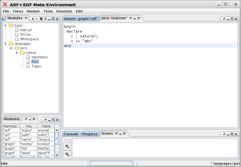
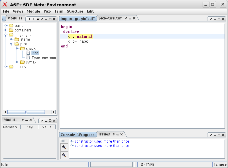
Now start typing the following (syntactically correct) Pico program:
begin declare x : natural; x := "abc" end
The result is shown in the Figure 1.9, “First program after typing it in.”.
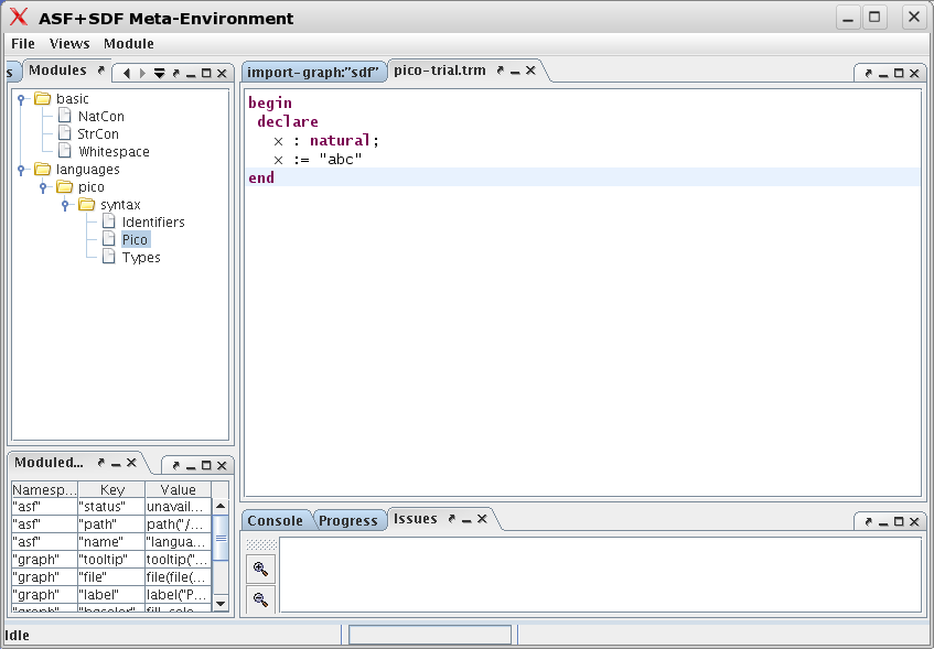
Next, goto to the menu and select the entry (or, alternatively, type Ctrl-S). The result is that the file is saved and parsed. As a result, all keywords will be highlighted as shown in Figure 1.10, “First program after saving it.”.
The syntax of Pico illustrates the following points:
-
All modules for a syntax definition reside in a subdirectory named
syntax. -
The main module of the syntax definition has the same name as the language (with an uppercase, since all module names start with an uppercase letter).
-
The modules
languages/pico/syntax/Identifiers,languages/pico/syntax/Typesandlanguages/pico/syntax/Picodefine (together with the modules they import) the syntax of the Pico language. -
This syntax can be used to:
-
Generate a parser that can parse Pico programs.
-
Generate a syntax-directed editor for Pico programs (including keyword highlighting).
-
Generate a parser that can parse equations containing fragments of Pico programs. This is similar to the use of different syntaxes in the definition of the
Booleansdescribed in the section called “basic/Booleans” and is used for program analysis and transformation.
-
In the syntax rules we have seen so far, many different symbols are used. Elementary symbols are:
-
Literal strings like
"begin"or"+". -
Sort names like
PROGRAMandSTATEMENT. Note that sorts are usually called non-terminals. -
Character classes like
[a-z]. Character classes can be combined using the following operators:-
~: complement. -
/: difference. -
/\: intersection. -
\/: union.
-
Complex symbols are:
-
Repetition:
-
S*: zero or more timesS. -
S+: one or more timesS. -
{S1 S2}*: zero or more timesS1separated byS2. -
{S1 S2}+: one or more timesS1separated byS2.
Repetition is best understood by the following examples (assuming the rule
"a" -> A):-
Aacceptsa. -
A+acceptsa,andaa, and .... -
{A ";"}+acceptsa, anda;a, anda;a;a, and ... but not:a;a;a;.
Slightly different patterns can be defined as well (using grouping and alternative as defined below):
-
(
A ";")+acceptsa;, anda;a;, anda;a;a;and ... but nota;a;a. -
(A ";"?)+acceptsa, anda a, anda;a, anda;a;, and ...
-
-
Grouping:
(S1 S2 ...)is identical toS1 S2 .... -
Optional:
S?: zero or one occurrence ofS. -
Alternative:
S | T: anSor aT. -
Tuple:
<S,T>: shorthand for"<" S "," T ">". -
Parameterized sort:
S[[ P1, P2 ]]
The general form of a grammar rule is:
S1 S2 ... Sn -> S0 Attributes
Where S1, ... are symbols and
Attributes is a (possibly empty) list of attributes.
Attributes are used to define associativity (e.g,
left), constructor functions
(cons), and the like.
Lexical syntax and context-free syntax are similar but between the symbols defined in a context-free rule, optional layout symbols may occur in the input text. A context-free rule (like the one above) is equivalent to:
S1 LAYOUT? S2 LAYOUT? ... LAYOUT? Sn -> S0 Attributes
For most programming and application languages, it is not enough that programs are syntactically correct, i.e., that they strictly conform to the syntax rules of the language. In many cases, extra requirements are imposed on programs such as:
-
Variables have to be declared before they can be used.
-
The operands of operators have to be of certain types.
-
Procedures can only be called with parameters that correspond in number and type with the formal parameters with the procedure has been declared.
These extra requirements are usually called type constraints, typechecking rules, or static semantics. We illustrate these requirements for the case of Pico.
The typechecking rules for the Pico language are very simple:
-
The only types are
naturalandstring. -
All variables should be declared before use.
-
Left-hand side and right-hand side of an assignment statement should have equal type.
-
The test in while-statement and if-statement should be
natural. -
Operands of
+and-should benatural; their result is alsonatural. -
Operands of
||should bestring; the result is alsostring.
The task of a typechecker for Pico is to assert that a given Pico program complies with the above rules. The typechecker can be seen as a transformation from a Pico program to an error report.
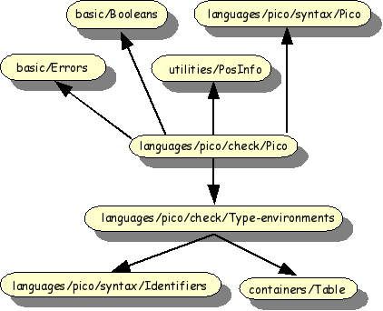
The import structure of the Pico typechecker is shown in Figure 1.11, “Import structure of Pico typechecker”.
The purpose of type environments is to maintain a mapping between identifiers and their type. This is done as follows:
module languages/pico/check/Type-environments imports languages/pico/syntax/Identifiers imports containers/Table[PICO-ID TYPE]
Notes:
| |
Import the library module |
| |
It is pragmatic to give a more descriptive name to
|
For convenience, we list the functions of Tables here:
module containers/Table[Key Value]
...
context-free
          syntax
"not-in-table" -> Value {constructor}
"new-table" -> Table[[Key,Value]]
lookup(Table[[Key,Value]], Key) -> Value
store(Table[[Key,Value]], Key,
Value) -> Table[[Key,Value]]
delete(Table[[Key,Value]], Key) -> Table[[Key,Value]]
element(Table[[Key,Value]], Key) -> Boolean
keys(Table[[Key,Value]]) -> List[[Key]]
values(Table[[Key,Value]]) -> List[[Value]]
...
In the case of Type-environments, the formal
parameter Key is bound to PICO-ID
and Value is bound to TYPE.
The central idea of the Pico typechecker is to visit all language constructs in a given Pico program while maintaining a type environment that maps identifiers to their declared type. Whenever an identifier is used, the type correctness of that use in the given context is checked against its declared type that is given by the type environment. An error message is generated when any violation of the type rules is detected. The following type checker is realistic in the following sense:
-
It discovers all errors.
-
It generates a message for each error.
-
The error message contains the source code location of the Pico construct that violates the type rules.
-
The type checker can be directly embedded in and used from The Meta-Environment.
First consider the syntax part of the Pico typechecker:
module languages/pico/check/Pico imports basic/Booleans imports basic/Errors
Notes:
| |
The library module |
| |
The library module |
| |
|
| |
Several auxiliary functions are defined that are used in the
definition of |
Now let's turn our attention to the equations part of the Pico typechecker:
equations [Main] start(PROGRAM, Program) =error("Expression should be of type natural", [localized("Expression", get-location(Exp))]) [default] tce(Exp, string, Tenv) = error("Expression should be of type string", [localized("Expression", get-location(Exp))]) [Tc7a] tce(Id, Type, Tenv) = when Type == lookup(Tenv, Id)
[Tc7b] tce(Nat-con, natural, Tenv) =
[Tc7c] tce(Str-con, string, Tenv) = [Tc7d] tce(Exp1 || Exp2, string, Tenv) = tce(Exp1, string, Tenv), tce(Exp2, string, Tenv)
[Tc7d] tce(Exp1 + Exp2, natural, Tenv) = tce(Exp1, natural, Tenv), tce(Exp2, natural, Tenv) [Tc7d] tce(Exp1 - Exp2, natural, Tenv) = tce(Exp1, natural, Tenv), tce(Exp2, natural, Tenv)
Notes:
| |
The first equation of this module is probably also the most
intimidating one. Its role is similar to the
|
| |
Type checking a complete program amounts to typechecking its declarations (this yields a type environment) and then checking its statements in that environment. |
| |
To type check declarations create a new type environment
( |
| |
To check a list of identifier-type pairs, we have to visit
each pair in the list. We use list matching
to achieve this: in the left-hand side |
| |
The left-hand side |
| |
An identifier that does not yet occur in the type environment is stored in the type environment together with its type. |
| |
Again, list matching to decompose a list of statements into a first statement and a list of remaining statements. Next, check the first statement and the remaining statements. |
| |
Check an assignment statement and discover that the identifier on the left-hand side of the assignment is not declared. Return an error. |
| |
Otherwise, check the type of the expression on the
right-hand side of the assignment. The declared type of the
variable on the left-hand side and the derived type of the
expression on the right-hand side should be the same. Note that
the |
| |
Checking if-statements and while-statements amounts to
checking that the test is of type
|
| |
Two default equations that generate an error message when the expected type and the actual type of an expression are unequal. |
| |
When the declared type of an identifier is equal to the expected type, we generate an empty list of errors. |
| |
Similarly, natural constants and string constants satisfy the expected types natural, respectively, string. |
| |
For operators, the operands are checked separately. |
Restart The Meta-Environment and do the following:
-
Open the menu and select .
-
In the dialog select
ASF+SDF Libraryto look for modules. -
Select succesively the directories
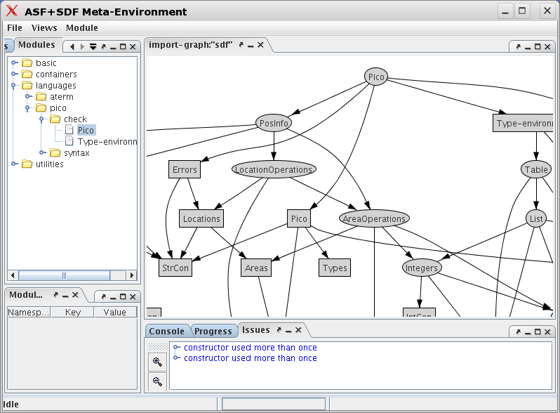
languages,pico,check, and then finally the modulePico.sdf. This is the top level module of the Pico typechecker. -
After some processing the screen results shown in Figure 1.12, “After opening languages/pico/check/Pico”.
The display of the import graph can be changed in various ways:
-
Left click and drag on the display to move to other parts of the import graph.
-
Right click on the display to adjust the size of the graph to let it fit on the display.
Now select languages/pico/check/Pico (in the
Modules panel on the left or in the import graph)
and open our previously created Pico program
pico-trial.trm over it (by right clicking on it,
following the pop-up menus, and opening
pico-trial.trm). Click somewhere in pico-trial.trm
and observe that several term editing menus have appeared. Of particular
interest is the menu labelled , see Figure 1.13, “Opening trial term over module
languages/pico/check/Pico”.
Important
The version of The meta-Environment produced to create these screen dumps gives two messages "constructor used more than one". Ignore them.
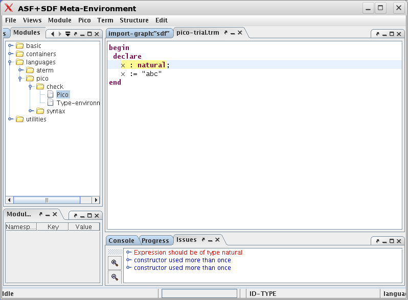
The final step is now to open the menu and
to select the button. The effect is
that the trial Pico program will be type checked and that an error
message will be displayed. Recall that the typecheck function
tcp is invoked with the current Pico program as
argument and is then reduced. See Figure 1.14, “After pushing the button in
the menu”.
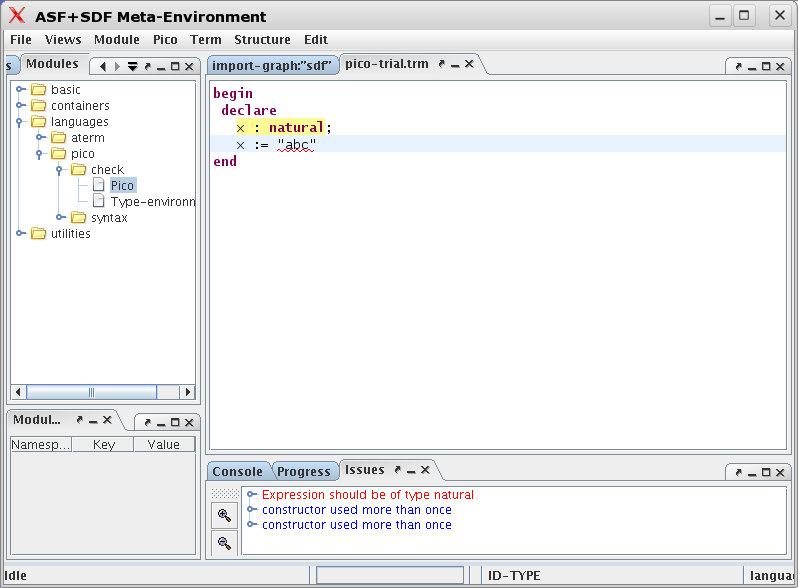
The error message is more informative than it seems: unfolding it reveals the location of the error. Just click on the message to highlight the error in the source code. That is shown in Figure 1.15, “Click on the error message to highlight its source”.
The Pico typechecker illustrates the following points:
-
ASF+SDF can be used to define a type checker.
-
ASF+SDF provides support for error messages and source code locations.
-
All modules for a typechecker reside in a subdirectory named
check. -
A typechecker can be integrated with The Meta-Environment. It is activated via the button.
-
Error messages are linked back to locations in the source text.
In addition to syntax rules and typechecking rules, most languages also need evaluation rules that determine how a program is to be executed. Execution amounts to taking a program and all its input and computing the program's result by a step-by-step execution of the statements in the program.
The evaluation rules for the Pico language are simple:
-
Variables of type
naturalare initialized to 0. -
Variables of type
stringare initialized to the empty string. -
A variable evaluates to its current value.
-
The variable on the left-hand side of an assignment statement gets as value the value that results from evaluating the expression on the right-hand side of the assignment.
-
If the test in an if-statement or while-statement evaluates to 0, this is interpreted as false.
-
Conversely, if the test in an if-statement or while-statement evaluates to a value unequal to 0, this is interpreted as true.
-
The statements in a list of statements are evaluated in sequential order.
The task of the Pico evaluator is to reduce a Pico program to the output it generates, in this case a value environment. The Pico evaluator can be seen as a transformation from a Pico program to its output.
The import structure of the Pico evaluator is shownin Figure 1.16, “Import structure of Pico evaluator”.
The sort VALUE is simply a container for
integer and string constants and is defined as follows:
module languages/pico/run/Values

imports basic/Integers basic/StrCon

exports
  sorts VALUE
  context-free syntax
    Integer     -> VALUE
    StrCon      -> VALUE
    "nil-value" -> VALUE
Notes:
| |
It would be better to use here |
| |
The constant |
The purpose of value environments is to maintain a mapping between identifiers and their current value. This is done as follows:
module languages/pico/run/Value-environments

imports languages/pico/syntax/Identifiers
imports languages/pico/run/Values
imports containers/Table[PICO-ID VALUE]

exports
  sorts VENV
  aliases
    Table[[PICO-ID, VALUE]] -> VENV
After the discussion of Type-environments in
the section called “languages/pico/check/Type-environments” this definition should be
easy to follow.
The central idea of the Pico evaluator is to first visit the declarations and initialise the declared variables. Next, the statements are visited one-by-one and their effect on the value environment is computed. The final value environment is then returned as the result of evaluation.
The syntax part of the Pico evaluator looks as follows:
module languages/pico/run/Pico

imports languages/pico/syntax/Pico
imports languages/pico/run/Value-environments
imports basic/Strings

exports

  context-free syntax
    "evp"(PROGRAM)                -> VENV

  context-free syntax
    "evd"(DECLS)                  -> VENV
    "evits"({ID-TYPE  ","}*)      -> VENV
    "evs"({STATEMENT ";"}*, VENV) -> VENV
    "evst"(STATEMENT, VENV)       -> VENV
    "eve"(EXP, VENV)              -> VALUE

hiddens
  imports basic/Comments
  context-free start-symbols
    VALUE-ENV PROGRAM

  variables
    "Decls"[0-9\']*   -> DECLS
    "Exp"[0-9\']*     -> EXP
    "Id"[0-9]*        -> PICO-ID
    "Id-type*"[0-9]*  -> {ID-TYPE ","}*
    "Nat"[0-9\']*     -> Integer
    "Nat-con"[0-9\']* -> NatCon
    "Series"[0-9\']*  -> {STATEMENT ";"}+
    "Stat"[0-9\']*    -> STATEMENT
    "Stat*"[0-9\']*   -> {STATEMENT ";"}*
    "Str" "-con"? [0-9\']* -> StrCon
    "Value"[0-9\']*   -> VALUE
    "Venv"[0-9\']*    -> VENV
    "Program"[0-9\']* -> PROGRAM
Having seen the syntax part of the Pico typechecker there are no
surprises here. The top level function evp maps
programs to value environments and needs some auxiliary functions to
achieve this.
The equations part of the Pico evaluator:
equations

[Main] start(PROGRAM, Program) =
       start(VENV, evp(Program))

equations

[Ev1]  evp(begin Decls Series end) =
       evs(Series, evd(Decls))

[Ev2]  evd(declare Id-type*;) = evits(Id-type*)

[Ev3a] evits(Id:natural, Id-type*) =
       store(evits(Id-type*), Id, 0)

[Ev3b] evits(Id:string, Id-type*) =
       store(evits(Id-type*), Id, "")

[Ev3c] evits() = []

[Ev4a] Venv' := evst(Stat, Venv),
       Venv'' := evs(Stat*, Venv')
       =================================
       evs(Stat ; Stat*, Venv) =  Venv''

[Ev4b] evs( , Venv) = Venv

[Ev5a] evst(Id := Exp, Venv) =
       store(Venv, Id, eve(Exp, Venv))

[Ev5b]             eve(Exp, Venv) != 0
       =================================================
       evst(if Exp then Series1 else Series2 fi, Venv) =
       evs(Series1, Venv)

[Ev5c]             eve(Exp, Venv) == 0
       =================================================
       evst(if Exp then Series1 else Series2 fi, Venv) =
       evs(Series2, Venv)

[Ev5d]           eve(Exp, Venv) == 0
       ==========================================
       evst(while Exp do Series od, Venv) =  Venv

[Ev5e] eve(Exp, Venv) != 0,  Venv' := evs(Series, Venv)
       ================================================
       evst(while Exp do Series od, Venv) =
       evst(while Exp do Series od, Venv')

[Ev6a] eve(Id, Venv) = lookup(Venv, Id)
[Ev6b] eve(Nat-con, Venv) = Nat-con
[Ev6c] eve(Str-con, Venv) = Str-con

[Ev6d] Nat1 := eve(Exp1, Venv),
       Nat2 := eve(Exp2, Venv)
       ====================================
       eve(Exp1 + Exp2, Venv) = Nat1 + Nat2

[Ev6e] Nat1 := eve(Exp1, Venv),
       Nat2 := eve(Exp2, Venv)
       ======================================
       eve(Exp1 - Exp2, Venv) =  Nat1 -/ Nat2

[Ev6f] Str1 := eve(Exp1, Venv),
       Str2 := eve(Exp2, Venv),
       Str3 := concat(Str1, Str2)
       ==============================
       eve(Exp1 || Exp2, Venv) = Str3

[default-Ev6]
       eve(Exp,Venv) = nil-value
Notes:
| |
A start equation that connects the functions defined here to
The Meta-Environment: given a program, a value environment is
returned and this is computed by applying the function
|
| |
Here declared variables are initialized. |
| |
Evaluation of a series of statements. Observe how the value
environment |
| |
Evaluation of if statement; the true case. |
| |
Evaluation of if statement; the false case. |
| |
Evaluation of while statement; the false case. |
| |
Evaluation of while statement; the true case. Note that the
body of the while statement is evaluated and that the resulting
value environment |
| |
A variable evaluates to its current value. |
| |
Constants evaluate to themselves. |
| |
Operators are evaluated by first evaluating their arguments
and then applying the relevant operator to them. Observe that the
|
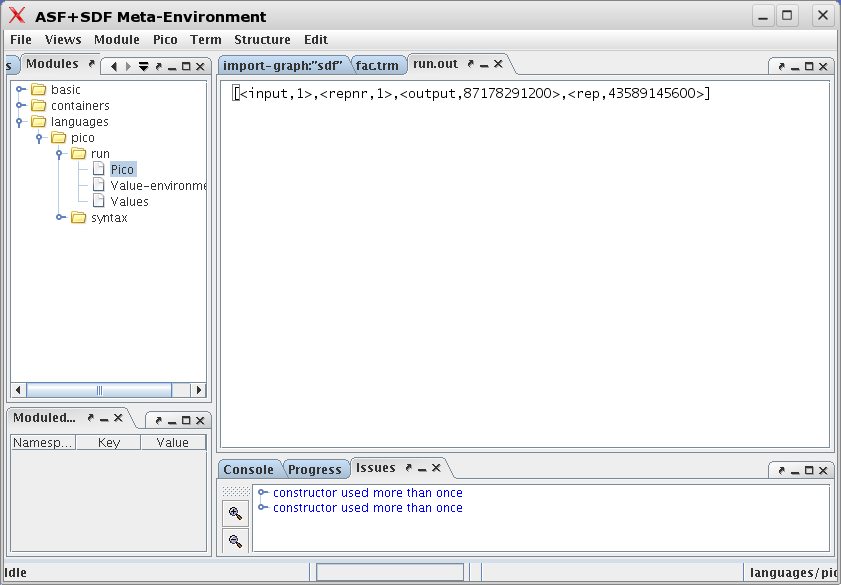
Now apply the evaluator function evp to our
Pico factorial example:
evp(
begin declare input : natural,
                      output  :  natural,
                      repnr: natural,
                     rep: natural;
          input := 14;
          output := 1;
          while input - 1 do
              rep := output;
              repnr := input;
              while repnr - 1 do
                 output := output + rep;
                 repnr := repnr - 1
              od;
              input := input - 1
          od
end
)
The result is:
[<input,1>,
<repnr,1>,
<output,87178291200>,
<rep,43589145600>]
To evaluate a Pico program perform the following steps:
-
Open the module
languages/pico/run/Pico.sdffrom theASF+SDF Library. -
Open the Pico program
fac.trmover this module. -
Open the menu and to select the button. The program is evaluated and the result is shown in a new editor pane called
run.out. This may take a while!
The result is shown in Figure 1.17, “After running the factorial program.”.
Important
Here again, more warnings appear. They can be ignored.
A compiler transforms a program in some higher level language (in this case Pico) to a lower level, in most cases assembly language. We will first define the assembly language and then define the transformation rules from Pico to assembly language. The overall import structure is shown in Figure 1.18, “Import structure Pico compiler”
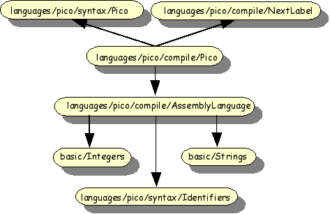
Now we define an assembly language for a stack-based CPU:
module languages/pico/compile/AssemblyLanguage

imports basic/Integers basic/Strings
imports languages/pico/syntax/Identifiers

exports
  sorts Label Instr
  lexical syntax
    [a-z0-9]+         -> Label

  context-free syntax
    "dclnat" PICO-ID  -> Instr
    "dclstr" PICO-ID  -> Instr

    "push" NatCon     -> Instr
    "push" StrCon     -> Instr
    "rvalue" PICO-ID  -> Instr
    "lvalue" PICO-ID  -> Instr
    "assign"          -> Instr
    "add"             -> Instr
    "sub"             -> Instr
    "conc"            -> Instr
    "label" Label     -> Instr
    "goto" Label      -> Instr
    "gotrue" Label    -> Instr
    "gofalse" Label   -> Instr
    "noop"            -> Instr

  sorts Instrs
context-free syntax
    {Instr";"}+       -> Instrs
Notes:
| |
Define an instruction label. |
| |
Directives to allocate a variable of type
|
| |
Push a natural constant or a string constant on the stack. |
| |
Push the value of a variable on the stack. |
| |
Push the name of a variable on the stack |
| |
Assign to a variable. The top entries on the stack are the value to be assigned and the name of the variable. Both are removed after executing this instruction. |
| |
The three operators for addition, subtraction and concatenation. They expect two values on the stack and replace them by the result of the operation. |
| |
Declare a label. This can be a target of one of the goto instructions. |
| |
Goto statements. The unconditional jump
( |
| |
A dummy instruction. |
| |
A list of instructions separated by semicolons. |
During code generation for if-statement and while-statement, the
need will arise to generate new labels to describe the control flow that
is implied by these statements. The function
nextlabel defined below describes this.
The syntax part looks as follows:
module languages/pico/compile/NextLabel

imports languages/pico/compile/AssemblyLanguage

exports
context-free syntax
  "nextlabel" "(" Label ")" -> Label

hiddens
lexical variables
  "Char+" [0-9]* -> [a-z0-9]+
Notes:
| |
The function |
| |
The definition uses a so-called lexical variable. Ordinary variables range over the subtrees (or subterms, if you prefer) of a term. In some cases it is necessary to be able to even inspect the contents of the lexical entities that form the leaves of a tree. Examples are identifiers, string constants and sometimes even the layout. Here we want to inspect the textual content of labels and define a lexical variable that ranges over the same lexical syntax as labels. |
The equations part:
equations

 [1] nextlabel(label(Char+)) = label(Char+ x)
This single equation decomposes a given label into a list of
characters. Next, it creates a new label consisting of the original list
of characters extended with a single character x.
Note that for every lexical sort (here: Label) there
exits an automatically generated constructor function (here:
label) that can be used to access the characters of a
lexical value or to construct a new one. The former happens at the
left-hand side of the above equation, the latter on the right-hand side.
Also observe that this is completely type safe and that only
syntactically correct lexical values can be constructed in this
way.
The goal of the Pico compiler is to translate a Pico program into an equivalent assembly language program.
The syntax part of the Pico compiler:
module languages/pico/compile/Pico

imports languages/pico/syntax/Pico
imports languages/pico/compile/AssemblyLanguage
imports languages/pico/compile/NextLabel


exports
  context-free syntax
    trp( PROGRAM ) -> Instrs

hiddens
  context-free start-symbols
    PROGRAM Instrs
  context-free syntax
    trd(DECLS)                   -> {Instr ";"}+
    trits({ID-TYPE  ","}*)       -> {Instr ";"}+
    trs({STATEMENT ";"}*, Label) -> <{Instr ";"}+, Label>
    trst(STATEMENT, Label)       -> <{Instr ";"}+, Label>
    tre(EXP)                     -> {Instr ";"}+

hiddens
  variables
    "Decls"[0-9\']*   -> DECLS
    "Exp"[0-9\']*     -> EXP
    "Id"[0-9]*        -> PICO-ID
    "Id-type*"[0-9]*  -> {ID-TYPE ","}*
    "Nat-con"[0-9\']* -> NatCon
    "Series"[0-9\']*  -> {STATEMENT ";"}+
    "Stat"[0-9\']*    -> STATEMENT
    "Stat*"[0-9\']*   -> {STATEMENT ";"}*
    "Str-con"[0-9\']* -> StrCon
    "Str"[0-9\']*     -> String

    "Instr*"[0-9\']*  -> {Instr ";"}+
    "Label" [0-9\']*  -> Label
    "Program"         -> PROGRAM
Notes:
| |
The main compiler function translates a Pico program into a sequence of instructions. |
| |
Auxiliary compiler functions. Observe that some of these
functions have the output sort |
The equations of the Pico compiler look as follows:
equations [main] start(PROGRAM, Program) =
Notes:
| |
The ubiquitous start equation that establishes that trees of
sort |
| |
A Pico program is compiled by first compiling its
declarations and then its instructions. The resulting instruction
sequences are then concatenated and returned as result. Note that
the translation of the series part of the program starts using the
label |
| |
Compile the declarations. |
| |
Compile an (id, type) pair. Depending on the declared type,
we generate a |
| |
Compile a series of statements by first compiling the first one and then the rest. Observe the careful propagation of the label information. |
| |
An empty series of statements is translated into a
|
| |
Compile an assignment statement. |
| |
Compile an if-statement. Labels are created to mark the instructions generated for the else branch and, respectively, the instructions following the code generated for the if statement. |
| |
Compile a while-statement. Two new label are generated to mark the instructions generated for the while statement and, respectively, the instructions following the code generated for the while loop. |
| |
Constants are compiled into appropriate push instructions. |
| |
Compilation of expressions. First compile both arguments (when the generated code is executed it leaves the two argument values on the stack) and then generate the appropriate operator instruction that will replace the two values on the stack by the result of the operator. |
Recall the Pico example that computes factorial and let's apply
the function trp to it:
trp(
begin declare input : natural,
                      output  :  natural,
                      repnr: natural,
                     rep: natural;
          input := 14;
          output := 1;
          while input - 1 do
              rep := output;
              repnr := input;
              while repnr - 1 do
                 output := output + rep;
                 repnr := repnr - 1
              od;
              input := input - 1
          od
end
)
The result is the following assembly language program:
        dclnat input;
        dclnat output;
        dclnat repnr;
        dclnat rep;
        noop; lvalue input;
        push 14;
        assign ;
        lvalue output;
        push 1;
        assign ;
        label xxxx;
        rvalue input; push 1; sub;
        gofalse xxxxx;
        lvalue rep;
        rvalue output;
        assign ;
        lvalue repnr;
        rvalue input;
        assign ;
        label xx;
        rvalue repnr; push 1; sub;
        gofalse xxx;
        lvalue output;
        rvalue output; rvalue rep; add;
        assign ;
        lvalue repnr;
        rvalue repnr; push 1; sub;
        assign ;
        noop;
        goto xx;
        label xxx ;
        lvalue input;
        rvalue input; push 1; sub;
        assign ;
        noop;
        goto xxxx;
        label xxxxx ;
        noop
TBD
Caution
compile does not generate a Pico menu entry but we need to use Reduce instead.
The Pico compiler illustrates the following issues:
-
ASF+SDF can be used to define a compiler.
-
ASF+SDF allows the decomposition of lexical values into characters and the construction of syntactically correct new lexical values.
-
Three languages are involved in the definition of the Pico compiler: ASF+SDF (the specification language), Pico (source language), and AssemblyLanguage (target language).
-
The compiler can be integrated in The Meta-Environment and is activated via the button.
As we have seen in the preceding examples, functions like typechecking, evaluation and compilation recursively visit all nodes in the parse tree of a program and perform their task at each node, being checking, evaluation or code generation. In these cases it is unavoidable that we need to define an equation for each possible language construct that has to be processed. The number of equations will then be at least equal to the number of grammar rules in the syntax of the language. In the case of real languages, like Java or COBOL, this amounts to hundreds and hundreds of syntax rules and by implication of hundreds of equations as well.
There are, fortunately, also many other applications where something interesting has to be done at only a few nodes. Examples are:
-
Computing program metrics like counting the number of identifiers, goto statements, McCabe complexity and the like.
-
Extracting function calls.
ASF+SDF provides traversal functions that automate these cases. There are two important aspects of traversal functions:
-
The kind of traversal:
-
accumulate a value during the traversal, this is indicated by:
traversal(accu). A typical example is a function that counts statements. -
transform the tree during the traversal, this is indicated by:
traversal(trafo). A typical example is a function that replaces certain statements. -
accumulate and transform at the same time, this is indicated by:
traversal(accu,trafo):
-
-
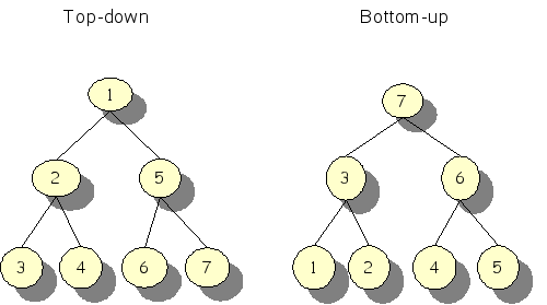
The order of traversal:
-
top-down versus bottom-up: In Figure 1.19, “Top-down versus bottom-up” the difference is shown: a top-down traversal starts with the root node and then traverses the root's children from the left to right, and so on. A bottom-up traversal, however, starts with the left-most leave of the tree and works its way up in the tree towards the root which is visited last.
-
break (stop at the first node where something can be done) or continue after visiting a node.
-
Consider the following very simple language of trees:
module Tree-syntax
imports Naturals
exports
  sorts TREE
  context-free syntax
    NAT           -> TREE
    f(TREE, TREE) -> TREE
    g(TREE, TREE) -> TREE
    h(TREE, TREE) -> TREE
  variables
    “N”[0-9]*     -> NAT
    “T”[0-9]*     -> TREE
Notes:
| |
The leaves of a tree are natural numbers. |
| |
The symbols |
| |
The variables |
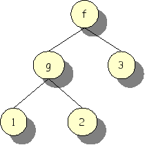
An example of a tree defined in this way is f(g(1,2),
3). Graphically, it looks as in Figure 1.20, “Example f(g(1,2),3) as tree”.
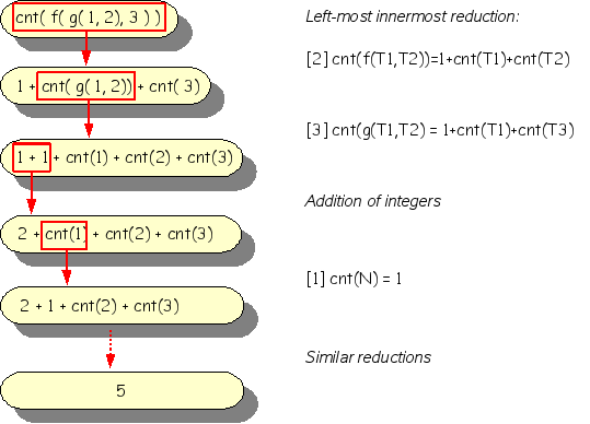
The classical solution for counting the nodes in a tree is as follows:
module Tree-cnt imports Tree-syntax exports context-free syntax cnt(TREE) -> NAT
Notes:
| |
The function |
| |
Visiting a leaf (a number) counts for one. |
| |
Visiting a non-leaf counts for one (this node) plus the counts for the left and the right subtree. An equation is needed for every constructor in the tree language. |
Counting the nodes of our previous example is achieved as follows:
cnt(f(g(1, 2), 3))
and returns:
5
The steps to arrive at this result are shown in Figure 1.21, “Reducing cnt(f(g(1, 2), 3))”.
Let's now reformulate the node counting example using traversal functions:
module Tree-cnt
imports Tree-syntax
exports
 context-free syntax
    cnt(TREE, NAT) -> NAT {traversal(accu,
                                     bottom-up,
                                     continue)}
equations
[1] cnt(T, N) = N + 1
Notes:
| |
Define |
| |
A single equation is needed to count any node (both leaves and
complex nodes). The first argument |
Counting the nodes of the example
cnt( f( g( f(1,2), 3 ),
           g( g(4,5), 6 )),
       0)
gives:
11
Now we switch to a simple transformation example: given a tree construct a new one that is identical except that all values at the leaves are incremented by one. This is achieved as follows:
module Tree-inc
imports Tree-syntax
exports
context-free syntax
  inc(TREE) -> TREE {traversal(trafo,
                               bottom-up,
                               continue)}
equations
[1] inc(N) = N + 1
Notes:
| |
The transformer |
| |
The single equation that performs the replacement. Observe
that this equation only matches at nodes that contain an integer
(this is due to the |
The example:
inc( f( g( f(1,2),  3 ),
           g( g(4,5), 6 )) )
gives:
f( g( f(2,3), 4 ),
      g( g(5,6), 7 ))
Continuing the incrementing example, we now want to make the amount of the increment variable.
module Tree-incp
imports Tree-syntax
exports
context-free syntax
  inc(TREE, NAT) -> TREE {traversal(trafo,
                                    bottom-up,
                                    continue)}
equations
[1] inc(N1, N2) = N1 + N2
Notes:
| |
We define a new |
| |
The equation has to be adjusted as well. |
Example:
inc( f( g( f(1,2),  3 ),
           g( g(4,5), 6 )),
       7 )
Result:
f( g( f( 8,  9), 10),
      g( g(11,12),  13))
Performing replacements in trees is a frequently occurring operation. Typically, certain values in a tree have to be replaced by other ones. These values can be simple or complex. One can distinguish different forms of replacement:
-
Deep replacement replaces only occurrences close to the leaves of the tree.
-
Shallow replacement replaces only occurrences close to the root.
-
Full replacement replaces all occurrences in a tree.
These forms of replacement form a nice test case for traversal
functions and we will discuss each in detail. The task at hand will be:
perform a deep/shallow/full replacement of all function symbols
g by a new function symbol
i.
Deep replacement only replaces occurrences close to the leaves of the tree. This suggests a bottom-up approach where on each path from the root of the tree to each leaf, at most one replacement may occur. This is exactly what the break attribute of traversal function achieves.
module Tree-drepl imports Tree-syntax exports context-free syntax i(TREE, TREE) -> TREE
Notes:
| |
Add the additional tree constructor i to make examples slightly more interesting. |
| |
The function |
| |
The equation that performs the actual replacement: the
subtree |
An example:
drepl( f( g( f(1,2), 3 ),
          g( g(4,5), 6 )) )
results in:
f( i( f(1,2), 3 ),
     g( i(4,5), 6 ))
Indeed, only the deepest occurrences of g
have been replaced.
Shallow replacement only replaces occurrences close to the root of the tree. This suggests a top-down approach where on each path from the root of the tree to each leaf, at most one replacement may occur. This is exactly what the break attribute of traversal function achieves.
module Tree-srepl
imports Tree-syntax
exports
context-free syntax
   i(TREE, TREE)   -> TREE
   srepl(TREE)      -> TREE {traversal(trafo,
                                       top-down,
                                       break)}
equations
[1] srepl(g(T1, T2)) = i(T1, T2)
Notes:
| |
The function |
The example:
srepl( f( g( f(1,2), 3 ),
          g( g(4,5), 6 )) )
results in:
f( i( f(1,2), 3 ),
     i( g(4,5), 6 ))
As expected, only the outermost occurrences of
g have been replaced.
Full replacement replaces all occurrences in the tree. In this case, there is no difference between a top-down or a bottom-up approach. The continue attribute of traversal function achieves traversal of all tree nodes.
module Tree-frepl
imports Tree-syntax
exports
context-free syntax
   i(TREE, TREE)   -> TREE
   frepl(TREE)      -> TREE {traversal(trafo,
                                       top-down,
                                       continue)}
equations
[1] frepl(g(T1, T2)) = i(T1, T2)
The example
frepl( f( g( f(1,2), 3 ),
          g( g(4,5), 6 )) )
results in:
f( i( f(1,2), 3 ),
     i( i(4,5), 6 ))
Indeed, all occurrences of g have now been
replaced.
Now let's turn our attention to a real example of traversal functions. The problem is that COBOL75 has two forms of if-statement:
-
"IF" Expr "THEN" Stats "END-IF"? -
"IF" Expr "THEN" Stats "ELSE" Stats
          "END-IF"?
In other words, COBOL75 has an if-then statement and an
if-then-else statement and both end on an optional keyword
END-IF. This leads to the well known dangling else
problem that may cause ambiguities in nested if statements. Given
IF expr1 THEN
   IF expr2 THEN
      stats1
   ELSE
      stats2
Is this an if-then statement with an if-then-else statement as then branch as suggested by the following layout:
IF expr1 THEN
   IF expr2 THEN
      stats1
ELSE
   stats2
Or is it the other way around, an if-then-else statement with an if-then statement as then branch:
IF expr1 THEN
IF expr2 THEN
stats1
ELSE
stats2
This is utterly confusing and error-prone, therefore it is a good idea to add END-IF to all if-statement to indicate that either
IF expr1 THEN
   IF expr2 THEN
      stats1
   ELSE
      stats2
   END-IF
END-IF
or
IF expr1 THEN
   IF expr2 THEN
      stats1
   END-IF
ELSE
   stats2
END-IF
is intended.
The following excerpt from a real application achieves this:
module End-If-Trafo imports Cobol
Notes:
| |
Import the COBOL grammar. It is huge and consists of hundreds of syntax rules. |
| |
The transformer |
| |
Two equations define the transformation for an if-then,
respectively, an if-then-else statement with missing
|
It must be stressed that, due to the nesting of if-statements, such a kind of transformation can never be done by a tool that is based on lexical analysis alone. The enormous savings due to the use of traversal functions should also be stressed: only two equations suffice to define the required transformation. Compare this with the hundreds of equations that would have been needed without traversal functions.
To conclude these illustrations of the use of traversal functions, we reconsider the problem of Pico typechecking and present a completely alternative solution that does not use type environments. Given a Pico program, the overall approach is to remove those part that are type correct and to repeat this process as long as possible. A type correct program will hence be reduced to an empty program, while a type-incorrect program will be reduced to a program that precisely contains the incorrect statements. The replacement strategy is as follows:
-
Replace all constants by their type, e.g.,
3becomestype(natural). -
Replace all variables by their declared type, e.g.,
x + 3becomestype(natural) + type(natural). -
Simplify type correct expressions, e.g.,
type(natural) + type(natural)becomestype(natural). -
Remove all type correct statements, e.g.,
type(natural) := type(natural)is removed.
Consider the erroneous program:
begin
   declare x : natural,
                y : natural,
                s : string;
      x := 10; s := "abc";
      if x then
             x := x + 1
      else
             s := x + 2
      fi;
      y := x + 2;
end
(take a second to spot the error) will thus reduce to:
begin
  declare;
  type(string) := type(natural);
end
This style of type checking leads to descriptive messages concerning the cause of errors and is an alternative to the style where explicit error locations have to be taken into account in the specification.
The "funny" Pico typechecker is defined as follows:
module Pico-typecheck imports Pico-syntax exports context-free syntax type(TYPE) -> ID
Notes:
| |
First we have to extend the Pico syntax, to allow type
indications in the code. Here, we allow at every position where an
identifier may occur a type indication of the form
|
| |
The traversal function |
| |
Visit each variable declaration and use
|
| |
Replace constants and variables by their type. |
| |
Replace type-correct expressions by their type. |
| |
Remove type-correct expressions and statements. |
This intermezzo introduces the following points:
-
For tree traversals that have to do work at every node, it is unavoidable to write many equations to describe the traversal: at least one equation is needed for every rule in the grammar of the language in question. Examples are typechecking, evaluation and code generation.
-
Other applications only have to do work at a few types of nodes. This is exemplified by various forms of metrics calculation and fact extraction.
-
Traversal functions automate such applications: only equations are needed for the cases where real work has to be done at a node; the other cases are handled automatically.
-
An accumulator is a traversal function that computes a certain value during the traversal of the tree.
-
A transformer is a traversal function that transform the tree during the traversal.
-
An accumulating transformer combines these functionalities.
-
Traversal functions can traverse the tree from root to leaves (top-down) or from leaves to root (bottom-up).
-
Traversal functions can visit all nodes on each path from root to tree (continuous) or only the first matching node (break).
The goal of a fact extractor is to extract information from source files that can be used by later analysis tools. Fact extraction is tightly coupled to the requirements of the analysis tools and can differ widely per application. Here we show a simple fact extractor that extracts:
-
A control flow graph.
-
A statement histogram.
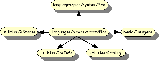
The import structure is shown in Figure 1.22, “Import structure Pico fact extractor”.
Two imported modules require explanation, but we do not go into too much details.
The module utilitities/Rstores defines
rstores, relation stores, that are used to maintain
mapping between a typed variable and a set or relation. Rstores are used
to collect the extracted facts and can be used later on by analysis tools.
Typical operations are:
-
create-store: create a new rstore. -
declare: define a new variable with its type and initial value. -
set: assign a value to a variable in the rstore.
The module utilities/Parsing defines parsing and
unparsing functions for values of specific sorts. The only function that
we will use is:
-
unparse-to-string: convert an arbitrary value (like an identifier, expression, or statement in a Pico program) to a string value. This conversion is necessary since sets and relations can only contain basic values like integers and strings and no complex values like fragments from parse trees.
The syntax definition of the Pico fact extractor:
module languages/pico/extract/Pico imports utilities/RStores imports languages/pico/syntax/Pico imports basic/Integers imports utilities/Parsing[PICO-ID]
Notes:
| |
The modules |
| |
Given a Pico program and an rstore, the function
|
| |
Similarly, function |
| |
These two functions are implemented using auxiliary traversal functions. |
| |
Variables can be annotated with the attributes
|
The equations for the Pico fact extractor:
equations

[main] Store1 := create-store(),
       Store2 := statementHistogram(Program, Store1),
       Store3 := controlFlow(Program, Store2)
       ===============================================
       start(PROGRAM, Program) = start(RStore, Store3)

equations

[hist] statementHistogram(Program, Store) =
       countStatements(Program,
                       declare(Store,
                               StatementHistogram,
                               rel[str,int]))

equations

[cS1] countStatements(Id := Exp, Store)  =
      inc(Store, StatementHistogram, "Assignment")

[cS2] countStatements(if Exp
                      then Stat*1
                      else Stat*2 fi,
                      Store) =
      inc(Store, StatementHistogram, "Conditional")

[cS3] countStatements(while Exp do Stat* od, Store) =
      inc(Store, StatementHistogram, "Loop")

equations

[cfg] Store1 := declare(Store,
                        ControlFlow,
                        rel[<str,loc>,<str,loc>]),
      <Entry, Rel, Exit> := cflow(Stat*)
      ============================================
      controlFlow(begin Decls Stat* end, Store) =
      set(Store1, ControlFlow, Rel)

equations

[cfg-1]
     <Entry1, Rel1, Exit1> := cflow(Stat),
     <Entry2, Rel2, Exit2> := cflow(Stat+)
     =====================================
     cflow(Stat ; Stat+) =
     <
      Entry1,
      union(Rel1, union(Rel2, product(Exit1, Entry2))),
      Exit2
     >

[cfg-2] cflow() = <{}, {}, {}>

equations

[cfg-3]
     <Entry, Rel, Exit> := cflow(Stat*),
     Control := <unparse-to-string(Exp),
                 get-location(Exp)>
     ==================================
     cflow(while Exp do Stat* od) =
     <
      {Control},
      union(product({Control}, Entry),
            union(Rel, product(Exit, {Control}))),
      {Control}
     >

[cfg-4]
     <Entry1, Rel1, Exit1> := cflow(Stat*1),
     <Entry2, Rel2, Exit2> := cflow(Stat*2),
     Control := <unparse-to-string(Exp),
                 get-location(Exp)>
     ==========================================
     cflow(if Exp then Stat*1 else Stat*2 fi) =
     <
      {Control},
      union(product({Control}, Entry1),
            union(product({Control}, Entry2),
                  union(Rel1, Rel2))),
      union(Exit1, Exit2)
    >

[default-cfg]
    Control := <unparse-to-string(Stat),
                get-location(Stat)>
    =========================================
    cflow(Stat) = <{Control}, {}, {Control}>
Notes:
| |
A start equation that links the extractor to the Meta-Environment: it creates a new rstore, fills it with the two defined extractions, and returns it as result. |
| |
Add a new variable |
| |
Perform the counting for three statement categories:
assignments, conditionals and loops. For each category a tuple of
the form |
| |
The function |
| |
The function cflow retruns a triple: the entry points, the internal control flow, and the exit points of the investigated language construct. In the case of a statement sequence, the exits of the first statement and the entries of the following statements have to be connected via a Carthesian product to create all possible control flow transfers between them. The internal relations Rel1 and Rel2 are added to this and the appropriate triple is returned. |
| |
A slightly more complex construction in order to cater for all control flows in a while loop. Observe that the control expression is the entry as well as the exit of the while-statement. Internally, the exits of the body of the loop have to be connected whith the control expression. |
| |
Here again, some plumbing is necessary to collect all the possible control flow from control expression, via then or else branch to the exits of the statement. |
To run a fact extraction on a Pico program perform the following steps:
-
Open the module
languages/pico/extract/Pico.sdffrom theASF+SDF Library. -
Open the term
fac.trmover this module (you may need to copy it first from this article or from theSDF Libraryin theexamplesdirectory). -
Open the menu and select the entry .
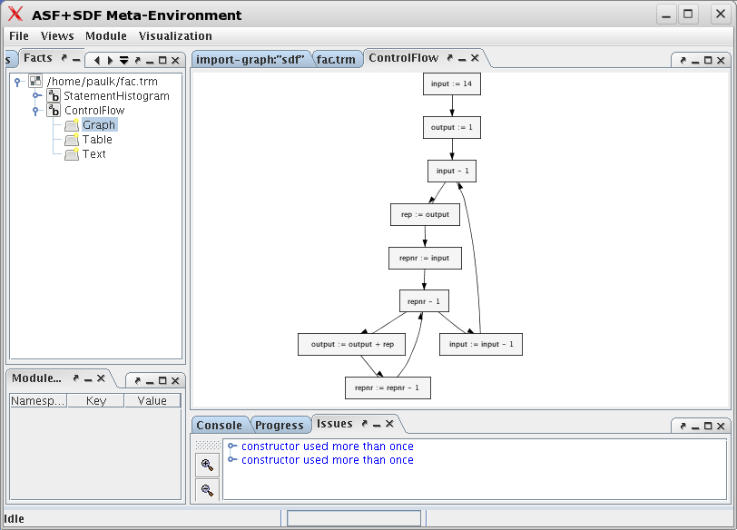
After some delay the extraction is complete (check, for instance,
the progress messages at the bottom of the window). The result is an
rstore that we can inspect with the fact browser that is available in
the left pane under Facts. For the various
variables in the rstore different visualisations are available (they
depend on the actual type of each variable). The effect of selecting the
graph visualization for the ControlFlow variable is
shown in Figure 1.23, “Graph display of ControlFlow”.
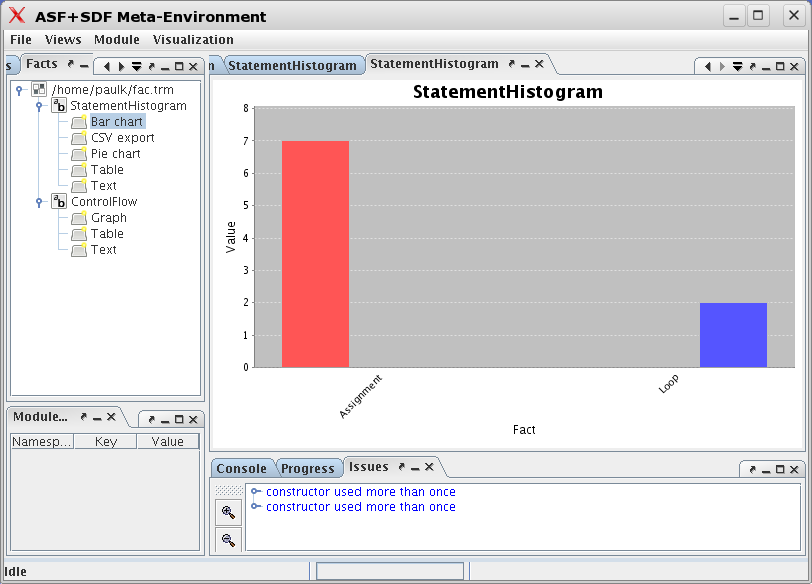
Another example is the visualization of the
StatementHistogram variable as bar chart shown in
Figure 1.24, “Bar chart display of StatementHistogram”.
The Pico extractor illustrates the following points:
-
Traversal functions are very useful for writing relatively short extraction functions.
-
Rstores can be used to represent extracted facts.
-
Fact extract can be integrated in The Meta-Environment and is activated via the button.
-
The Meta-Environment supports various visualizations for rstores.