The Language Specification Formalism ASF+SDF

ASF+SDF is intended for the high-level, modular, description of the analysis and transformation of computer-based formal languages. It is the result of the marriage of two formalisms ASF (Algebraic Specification Formalism) and SDF (Syntax Definition Formalism). ASF+SDF can be used to implement compilers, refactoring tools, reverse engineering tools, re-engineering tools, etc. Basically all meta programs are within the scope of ASF+SDF. It is specifically designed to make the construction of meta programs more easy.

Key features of ASF:

There are two ways to write ASF+SDF specifications and to execute them:

SDF is used to describe syntax of (programming) languages using context-free production rules. The parsers generated by SDF produce parse trees. The nodes of the parse trees are the productions of the SDF specification. The leaves of the parse trees are the characters of the input text. ASF programs take parse trees as input and produce parse trees as output. A node in the parse tree is a "function" for ASF. All ASF does is replace functions by other functions, generating a new parse tree that can be unparsed to obtain an output text.

ASF stands for Algebraic Specification Formalism. This paragraph describes ASF in terms of algebras. ASF can be used to define many-sorted algebra's. Many sorted algebra's have so-called signatures to describe the shape of algebraic terms. In ASF we use SDF to describe the signature of terms. An SDF production is an ASF term constructor. A non-terminal in SDF is an algebraic sort in ASF. ASF specification are collections of equations. The algebraic equations define which terms are equal to which other terms. This is where the algebra stops, and term rewriting begins. In fact the equations are interpreted as rewrite rules. Each pattern on the left-hand side is searched in the input term, and replaced by the right-hand side.

The parse trees of SDF contain the full input program text and all SDF productions that have been used to parse it. ASF provides full access to all details of the parse tree, such that any analysis or transformation is possible.

Parse trees and abstract syntax trees are very complicated structures. In ASF you do not have to deal with this complexity. Parse tree patterns are expressed in the programming language that is analyzed or transformed. This is called "concrete syntax". ASF rewrites parse trees to other parse trees under the hood, but the programmer types in source code of the language analyzed or transformed. This manual contains many examples of this.

ASF+SDF uses the module mechanism provided by SDF. Each module M in an SDF specification is stored in a file M.sdf. To each module M one can simply add equations as needed by providing them in a file M.asf. The result is an ASF+SDF specification. We call M.sdf the SDF part of module M and M.asf the ASF part of M.

Note that some of the semantics of ASF is triggered by the attributes of productions in SDF. The {bracket} attribute is one example, another important example is the {traversal(...)} attribute.

The variables and lexical variables sections of SDF are important. In these sections you describe the syntax of meta variables. These are exactly the variables used in the concrete syntax patterns used in ASF to construct and deconstruct source code.

This document describes the syntax of ASF and its semantics. The syntax of ASF is structured as follows:

Figure 1.1. Syntactic structure of ASF

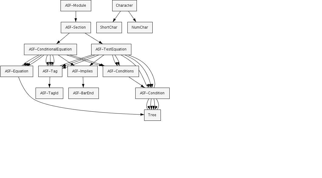
We will now describe the ingredients of the ASF part of modules. Each module contains any number of sections. There are equations sections and tests sections. The equations sections contain normal equations and conditional equations. The tests sections contain normal tests and conditional tests. The document is split into three parts. First we discuss the basic features of ASF+SDF, then we discuss the advanced features of ASF+SDF. Note that both the syntax and the name of the Tree non-terminal from the above picture is defined by the programmer in SDF. It will be different for every ASF+SDF program.

We conclude the description of ASF+SDF with Historical notes and bibliographic background on ASF+SDF

Equations are always contained in an equations section that has the following structure:

equations
    <Equation>*

In other words, the keyword equations followed by zero or more equations. These may be unconditional or conditional equations as described below.

An unconditional equation has the form

[<TagId>] <Term> = <Term>

where <TagId> is the name of the equation. It is a sequence of letters, digits, and/or minus signs (-) starting with a letter or a digit. Next follows an equality between two <Term>s. A <Term> is any string described by the SDF part of the module in which the equation occurs. There are some restrictions on the terms in an equation:

It is assumed that the variables occurring in the equation are universally quantified. In other words, the equality holds for all possible values of the variables.

An unconditional equation is a special case of a conditional equation, i.e., an equality with one or more associated conditions (premises). The equality is sometimes called the conclusion of the conditional equation. In ASF+SDF a conditional equation can be written in three (syntactically different, but semantically equivalent) ways. Using when

[<TagId>]  <Term1> = <Term2> when <Condition1>, <Condition2>, ...

or using an implication arrow ===>

[<TagId>]  <Condition1>, <Condition2>, ... ===> <Term1> = <Term2>

or using a horizontal bar

[<TagId>]  <Condition1>, <Condition2>, ... 
           ===============================
                 <Term1> = <Term2>

where <Condition1>, <Condition2>, ... are conditions which may be of one of the following forms:

The conditions of an equation are evaluated from left to right. Let, initially, Vars be the set of variables occurring in the left-hand side of the conclusion of the equation.

Match conditions are evaluated as follows. The left-hand side of a match condition must contain at least one new variable not in Vars. Reduce the right-hand side of the match condition to a normal form. The match condition succeeds if this normal form and the left-hand side of the condition match. The new variables resulting from this match are added to Vars and bound to the corresponding parts of the right-hand side of the condition.

For the evaluation of each equality condition we require that the condition contains only variables in Vars. Reduce both sides of the condition to normal form and the condition succeeds if both normal forms are identical. Technically, this is called a join condition. The evaluation of negative conditions is described by replacing in the above description ``identical'' and ``match'' by ``not identical'' and ``do not match'', respectively.

After the successful evaluation of the conditions, all variables occurring in the right-hand side of the conclusion of the equation should be in Vars. New variables (see above) should therefore not occur on both sides of a positive condition, in a negative condition, or in the right-hand side of the conclusion.

In the ASF+SDF Meta-Environment, equations can be executed as rewrite rules. This can be used to reduce some initial closed term (i.e., not containing variables) to a normal form (i.e., a term that is not reducible any further) by repeatedly applying rules from the specification. A term is always reduced in the context of a certain module, say M. The rewrite rules that may be used for the reduction of the term are the rules declared in M itself and in the modules that are (directly or indirectly) imported by M. The search for an applicable rule is determined by the reduction strategy, that is, the procedure used to select a subterm for possible reduction. In our case the leftmost-innermost reduction strategy is used. This means that a left-to-right, depth-first traversal of the term is performed and that for each subterm encountered an attempt is made to reduce it. Next, the rules are traversed one after the other. The textual order of the rules is irrelevant, but default equations come last.

If the selected subterm and the left-hand side of a rule (more precisely: of the left-hand side of its conclusion) match, we say that a redex has been found and the following happens. The conditions of the rule are evaluated and if the evaluation of a condition fails, other rules (if any) with matching left-hand sides are tried. If the evaluation of all conditions succeeds, the selected subterm is replaced by the right-hand side of the rule (more precisely: the right-hand side of the conclusion of the rule) after performing proper substitutions. Substitutions come into existence by the initial matching of the rule and by the evaluation of its conditions. For the resulting term the above process is repeated until no further reductions are possible and a normal form is reached (if any).

We give here a number of elementary examples with the sole purpose to illustrate a range of features of ASF+SDF:

For larger and more interesting examples, we refer to ASF+SDF by Example. Add link.

Addition and Multiplication on Numerals

The natural numbers 0, 1, 2, ... can be represented in a form that is more convenient for formal reasoning:

• 0 is represented by 0.

• 1 is represented by succ(0).

• 2 is represented by succ(succ(0)).

• ...

• The number N is represented by succN(0), i.e., N applications of succ to 0.

Let's first formalize the grammar of these numerals in an SDF definition Numerals.sdf.

Example 1.1. Numerals.sdf

module Numerals
exports
 sorts NUM                   
 imports basic/Whitespace    
  context-free syntax
      "0"          -> NUM    
      succ(NUM)    -> NUM    
  context-free start-symbols
      NUM                    

Notes:

	Declares the sort NUM that will represent all numerals.
	Import the library module basic/Whitespace in order to define layout and comments.
	Define the constant 0.
	Define the successor function succ. Note that we use a prefix function here (see XXX); the unabbreviated definition would be "succ" "(" NUM ")" -> NUM
	Declare NUM as start symbol to enable the parsing of NUMs.

Having defined numerals, we can parse texts like 0, succ(0), etc. as syntactically correct NUMs.

The next step is to define addition and multiplication on numerals. Let's start with addition. We do this by introducing a module Adder.sdf that defines syntax for the add function.

Example 1.2. Adder.sdf

module Adder
exports
  imports Numerals                    
  context-free syntax
      add(NUM, NUM)  -> NUM            
  variables
      "X"            -> NUM           
      "Y"            -> NUM

Notes:

	Import the previously defined module Numerals.
	Define the syntax of the add function.
	Define the variables X and Y of sort NUM. They will be used in the equations.

Now we are ready for Adder.asf that defines the equations for the add function.

Example 1.3. Adder.asf: the ASF part of the Adder module

equations                             
[1] add(0, X) = X                     
[2] add(succ(X), Y) = succ(add(X,Y))  

Notes:

	The ASF part starts with the keyword equations.
	First equation: adding 0 to an arbitrary numeral X yields that same numeral.
	Adding Y to the successor of X is the same as applying the successor to the addition of X and Y.

After these preparations we can parse and reduce terms using the module Adder:

• The term 0 reduces to 0 in zero steps; no simplifications are possible.

• The term succ(0) reduces to succ(0) in zero steps; no simplifications are possible.

• The term add(succ(succ(0)), succ(succ(0))) reduces to succ(succ(succ(succ(0)))) in 3 steps; this corresponds to 2 + 2 = 4.

We complete this example with Multiplier.sdf and Multiplier.asf that define a multiplication operator on numerals as well.

Example 1.4. Muliplier.sdf

module Multiplier
exports
  imports Adder                       
  context-free syntax
    mul(NUM,NUM) -> NUM               

Notes:

	Import the module Adder that have just defined above.
	Define the syntax of the function mul.

The equations for mul are defined in Multiplier.asf.

Example 1.5. Multiplier.asf

equations
[1] mul(0, X) = 0                      
[2] mul(succ(X), Y) = add(mul(X,Y), Y) 

Notes:

	Multiplying any numeral by zero yields zero.
	Reduce multiplication to addition: multiplying Y by X+1 is the same as multiplying Y by X and then adding Y.

We can now parse and reduce terms using the module Multiplier:

• The term mul(succ(succ(succ(0))), succ(succ(0))) reduces to succ(succ(succ(succ(succ(succ(0)))))); this corresponds to 3 * 2 = 6.

Booleans

The Boolean constants true and false and the Boolean functions and, or and not are also completely elementary and therefore well-suited for illustrating some more features of ASF+SDF. The syntax of Booleans is given in Booleans.sdf.

Example 1.6. Booleans.sdf

module Booleans
exports
  sorts BoolCon                        
  context-free syntax
     "true"  -> BoolCon                
     "false" -> BoolCon

  sorts Boolean                        
  context-free start-symbols           
        Boolean
  context-free syntax
     BoolCon               -> Boolean  
     and(Boolean, Boolean) -> Boolean  
     or(Boolean,Boolean)   -> Boolean  
     not(Boolean)          -> Boolean  

hiddens                                
  imports basic/Comments               
  variables
     "B" -> Boolean                    

Notes:

	Introduce the sort BoolCon that will represent the constants true and false. It is good practice to define constants as a separate sort.
	Here are the definitions of the constants themselves.
	Introduce our sort of interest: Boolean.
	Since we will be dealing with Boolean terms, it is mandatory that they can be parsed. Hence we need to define a start symbol for them.
	Every Boolean constant BoolCon is a Boolean.
	Definition of the syntax of and, or and not.
	It is good practice to define comments (as needed in the equations) and variables as hidden. This has the advantage that comment conventions and variable declaration do propagate to the modules that import the current module.
	Import standard comments.
	Define the single variable B for later use in the equations.

After these preparations we are ready to parse Boolean terms like:

• true

• and(true,false)

• and(or(true,not(false)),true)

• or(true, B)

• and so on and so forth.

The definition of the functions on Booleans now simply requires writing down the truth tables in the form of equations and is given in Booleans.asf.

Example 1.7. Booleans.asf

equations

[or1] or(true, true)     = true
[or2] or(true, false)    = true
[or3] or(false, true)    = true
[or4] or(false, false)   = false

[and1] and(true, true)   = true
[and2] and(true, false)  = false
[and3] and(false, true)  = false
[and4] and(false, false) = false

[not1] not(true) = false
[not2] not(false) = true

We can now parse and reduce terms using Booleans:

• The term true reduces to true.

• The term and(true,false) reduces to false.

• The term and(or(true,not(false)),true) reduces to true.

As a final touch, a similar but shorter definition of the Boolean functions is possible. By using variable B, which we did declare but have not used so far, a shorter definition is possible see, for instance, the definition for or below.

Example 1.8. A shorter definition for or.

[or1'] or(true, B)  = true
[or2'] or(false, B) = B

Booleans with user-defined syntax

The Booleans we have seen in the previous example are fine, but the strict prefix notation makes Boolean terms less readable. Would it be possible to use more friendly notation like true & false instead of and(true, false) or true | false instead of or(true, false)? Can this be defined in ASF+SDF? The answers are yes and yes. In fact user-defined syntax is one of the unique features of ASF+SDF.

In FriendlyBooleans.sdf we show a version of the Booleans with user-defined syntax.

Example 1.9. FriendlyBooleans.sdf

module FriendlyBooleans
exports
  sorts BoolCon
  context-free syntax
     "true"  -> BoolCon
     "false" -> BoolCon

  sorts Boolean
  context-free start-symbols
        Boolean
  context-free syntax
     BoolCon               -> Boolean
     Boolean "&" Boolean   -> Boolean {left}     
     Boolean "|" Boolean   -> Boolean {left}
     not(Boolean)          -> Boolean            
     "(" Boolean ")"       -> Boolean {bracket}  
  context-free priorities                        
     Boolean "&" Boolean -> Boolean >
     Boolean "|" Boolean -> Boolean
hiddens
  imports basic/Comments
  variables
     "B" -> Boolean

Notes:

	Here the infix syntax for the and and or function is defined.
	Since we have infix functions, parentheses are needed for grouping.
	We keep the prefix version of the not function to illustrate the mixture of prefix and infix notation.
	A priority rules defines that & binds stronger than |.

After these preparations, the equations are shown in FriendlyBooleans.asf.

Example 1.10. FriendlyBooleans.asf

equations
[or1] true | B    = true
[or2] false | B   = B

[and1] true & B   = B
[and2] false & B  = false

[not1] not(true)  = false
[not2] not(false) = true

Important

Something interesting is going on here: we defined syntax rules in FriendlyBooleans.sdf and use them here in FriendlyBooleans.asf. This means that we use syntax in the equations that we have defined ourselves! Think about the implications of this: if we have an SDF definition for a programming language, we can easily write equations that contain programming language fragments. This unique feature makes ASF+SDF the ultimate language for writing program transformations.

Specification writers are supposed to make no errors, but we are all human. It is therefore convenient to explicitly state your expectations about the normal forms for some typical input terms. The tests in ASF+SDF provide a convenient way to document this and to run unit test for a module.

Tests are always contained in a tests section that has the following structure:

tests
    <Test>*

The global structure of the ASF part of a module then becomes:

equations
  <Equation>*
tests
  <Test>*

In fact, a module may contain an several test and equations sections in arbitrary order.

Each test has the form of a condition preceded by a label:

[<TagId>] <Condition>

A test may not contain variables and only the operators == and != can be used.

The tests for each module can be run via the check menu item in the user-interface of The Meta-Environment.

equations
 ... see List.asf ...

tests
 [sanity]      []                      != [1]
 [append1]     [1,2,3] ++ 4            == [1,2,3,4]
 [append2]     1 ++ [2,3,4]            == [1,2,3,4]
 [length1]     length([1,2,3])         == 3
 [is-element1] is-element(2, [1,2,3])  == true
 [is-element2] is-element(5, {1,2,3])) != true

As we have seen in Executing Equations, the evaluation strategy for normalizing terms given the equations is based on innermost rewriting. All equations have the same priority. Given the outermost function symbol of a redex the set of equations with this outermost function symbol in the left-hand side is selected and all these rules will be tried. However, sometimes a specification writer would like to write down a rule with a special status: try this rule if all other rules fail. A kind of default behaviour is needed. ASF+SDF offers functionality in order to obtain this behaviour. If the TagId of an equation starts with default- this equation is considered to be a special equation which will only be applied if no other rule matches.

module Types

imports basic/Whitespace
imports basic/Booleans

exports
  context-free start-symbols Type
  sorts Type

  context-free syntax
    "natural"     -> Type
    "string"      -> Type
    "nil-type"    -> Type
    compatible(Type, Type) -> Boolean

hiddens
  variables
    "Type"[0-9]*  -> Type

equations
[Type-1]  compatible(natural, natural) = true
[Type-2]  compatible(string, string)   = true
[default-Type] 
          compatible(Type1,Type2)      = false 

equations
[Type-1]  compatible(Type, Type)  = true
[default-Type] 
          compatible(Type1,Type2) = false 

equations
[Type-1]  compatible(Type, Type)  = true
[Type-2]       Type1 != Type2
          ===============================
          compatible(Type1,Type2) = false 

List matching, also known as associative matching, is a powerful mechanism to describe complex functionality in a compact way. Unlike the matching of ordinary (non-list) variables, the matching of a list variable may have more than one solution since the variable can match lists of arbitrary length. As a result, backtracking is needed. For instance, to match X Y (a list expression containing the two list variables X and Y indicating the division of a list into two sublists) with the list ab (a list containing two elements) the following three alternatives have to be considered:

In the unconditional case, backtracking occurs only during matching. When conditions are present, the failure of a condition following the match of a list variable leads to the trial of the next possible match of the list variable and the repeated evaluation of following conditions.

Example: Sets

Let's consider the problem of removing double elements from a list. This shown is in Sets.sdf and Sets.asf.

Example 1.16. Sets.sdf

module Sets
exports
  imports basic/Whitespace
  context-free start-symbols Set
  sorts Elem Set

  lexical syntax
    [a-z]+ -> Elem                

  context-free syntax
    "{" {Elem ","}* "}" -> Set    

hiddens
  variables
    "Elem"[0-9]*  -> Elem         
    "Elem*"[0-9]* -> {Elem ","}*  

Notes:

	This defines constants of sort Elem as a sequence of one or more lowercase letters.
	This defines the syntax of a Set: an opening curly bracket, a list of zero or more Elems separated by comma's, followed by a closing curly bracket. This is a typical syntax pattern; don't get confused by the different roles that the curly brackets play: the "{" and "}" are literal string that are part of the syntax of Sets, while {Elem ","}* describes a syntactic list of Elems separated by commas.
	This defines variables Elem1, Elem2 and so on of sort Elem.
	This defines variables Elem*1, Elem*2 and so on of sort {Elem ","}*. Observe the funny variable name containing the non-alphanumeric character *. Some ASF+SDF specification writers use the convention that variables that range over list sorts end on either * or + and maybe followed by digits. See How to name Variables.

We can now parse sets like:

• {}

• {a}

• {a, b}

• {a, b, c, d, e, f, g, h, i, j, k, l, m, n, o, p, q, r, s, t, u, v, w, x, y, z}

• and so on.

The actual solution of our problem, removing duplicates from a list, is shown in Sets.asf. Observe that the single equation has a left-hand side with two occurrences of variable Elem, so it will match on a list that contains two identical elements.

In the right-hand side, one of these occurrences is removed. However, this same equation remains applicable as long as the list contains duplicate elements.

Example 1.17. Sets.asf

equations
[set] {Elem*1, Elem, Elem*2, Elem, Elem*3} = 
      {Elem*1, Elem, Elem*2, Elem*3}

Important

This specification of sets is very elegant but may become very expensive to execute when applied to large sets. There are several strategies to solve this:

• Use ordered lists and ensure that the insert operation checks for duplicates.

• Use a more sophisticated representation like, for instance, a balanced tree.

Example: Lists

A sample of operations on lists of integers is shown in Lists.sdf and Lists.asf.

Example 1.18. Lists.sdf

module Lists

imports basic/Booleans
imports basic/Integers
imports basic/Whitespace

exports
  context-free start-symbols 
        Boolean Integer List             
  sorts List

  context-free syntax
    "[" {Integer ","}*  "]"   -> List    
    List "++" Integer         -> List    
    Integer "++" List         -> List    
    is-element(Integer, List) -> Boolean 
    length(List)              -> Integer 
    reverse(List)             -> List    
    sort(List)                -> List    

hiddens
  variables
    "Int"[0-9]*  -> Integer
    "Int*"[0-9]* -> {Integer ","}* 

Notes:

	In the context-free syntax below, we define functions with result sorts Boolean, Integer and List and all these sorts will probably occur in input terms. It is therefore a good idea to declare all these sort as start symbol.
	Define the syntax of lists of integers. Examples are: [] [1] [1, 3, 5, 7, 11]
	Append an integer to a list.
	Prepend an integer to a list.
	Check for element in list.
	Determine length of list.
	Reverse a list.
	Sort a list.

Given these syntax definitions, we can define the meaning of the various functions in Lists.asf.

Example 1.19. Lists.asf

equations
  [app-1] [Int*] ++ Int = [Int*, Int]                       
  [pre-1] Int ++ [Int*] = [Int, Int*]

  [len-1] length([]) = 0                                    
  [len-2] length([Int, Int*]) = 1 + length([Int*])

  [is-1] is-element(Int, [Int*1, Int, Int*2]) = true        
  [default-is]
         is-element(Int, [Int*]) = false

  [rev-1] reverse([]) = []                                  
  [rev-2] reverse([Int, Int*]) = reverse([Int*]) ++ Int

  [srt-1]            Int1 > Int2 == true                    
         =========================================
         sort([Int*1, Int1, Int*2, Int2, Int*3]) = 
         sort([Int*1, Int2, Int*2, Int1, Int*3])
  [default-srt]
         sort([Int*]) = [Int*]

Notes:

	The definition of the append and prepend operators ++ illustrates how list variables like Int* can be used to first extract elements from a list (on the left-hand side) and later insert them in a new list (on the right-hand side).
	The length function is defined by a simple induction on lists.
	The two occurrences of the variable Int in equation [is-1] illustrates the use of list matching for a search for a given element in a list.
	The reverse function is defined by recurring over the elements of the list. Note how the append operator ++ is used in equation [rev-2]. One can avoid using an auxiliary operator at the expense of introducing a condition and an extra variable: [rev-2'] [Int*1] := reverse([Int*]) =================================== reverse([Int, Int*]) = [Int*1, Int]
	The equations for the function sort show, once more, the expressive power of list matching: in the left-hand side of [srt-1] two elements Int1 and Int2 are picked and if Int1 is greater than Int2, the elements are swapped and sort is applied again.

Computations may contain unnecessary repetitions. This is the case when a function with the same argument values is computed more than once. Memo functions exploit this behaviour and can improve the efficiency of ASF+SDF specifications considerably. They are defined by adding a memo attribute to a function definition

Memo functions are executed in a special manner by storing, on each invocation, the set of argument values and the derived normal form in a memo table. On a subsequent invocation with given arguments, it is first checked whether the function has been computed before with those arguments. If this is the case, the normal form stored in the memo table is returned as value. If not, the function is normalized as usual, the combination of arguments and computed normal form is stored in the memo table, and the normal form is returned as value.

Adding a memo attribute does not affect the meaning of a function. There is, however, some overhead involved in accessing the memo table and it is therefore not a good idea to add the memo attribute to each function.

Example: Fibonacci

The Fibonacci function shown in Fib.sdf and Fib.asf below illustrates the use of memoization.

Example 1.20. Fib.sdf

module Fib

imports basic/Whitespace
imports Adder                 

exports
  context-free syntax
    fib(NUM)  -> NUM {memo}   

Notes:

	Import the module Adder we have seen before in the section Addition and Multiplication of Numerals.
	Define the syntax of the fib function. The memo attribute indicates that memoization should be used when executing this function.

The definition of the Fibonacci function fib is given in Fib.asf.

Example 1.21. Fib.asf

equations
[fib-0] fib(0)             = succ(0)
[fib-1] fib(succ(0))       = succ(0)
[fib-n] fib(succ(succ(X))) = add(fib(succ(X)), fib(X))

The resulting improvement in performance as follows:

Table 1.1. Execution times for the evaluation of fib(n)

fib(n)	Execution time without memo (sec)	Execution time with memo (sec)
fib(16)	2.0	0.7
fib(17)	3.5	1.1
fib(18)	5.9	1.8
fib(19)	10.4	3.3

Some functions symbols, like succ in the definition of Numerals cannot be reduced; they are constructors that are used to build the datastructures that are being defined. Other function symbols, like add and mul, are reducible; the equations define how these symbols can be removed from a term. There are currently, two ways to indicate that a function is a constructor:

This is a confusing state of affairs that should be repaired.

This section has still to be converted to V2.0: (a) Describe structured lexicals and give examples. (b) Split examples below in SDF and ASF part.

A context-free syntax rule describes the underlying tree structure. A lexical syntax rule defines in fact the underlying structure of the lexical tokens. Sometimes it is necessary to create or manipulate the characters of lexical tokens, for instance when converting one lexical entity into another. ASF+SDF provide the so-called lexical constructor functions to manipulate the characters of the lexical entities. Furthermore, ensure the lexical constructor functions that the underlying structure is not violated or that illegal lexical entities are created.

The only way to access the actual characters of a lexical token is by means of lexical constructor functions. For each lexical sort LEX a lexical constructor function is automatically derived as follows:

lex( LEX ) -> LEX

module Nats

imports basic/Whitespace

exports
  context-free start-symbols Nat-con
  sorts Nat-con

  lexical syntax
    [0-9]+ -> Nat-con 

hiddens
  lexical variables
    "Char+"[0-9]* -> [0-9]+
equations

  [1] nat-con(0 Char+) = nat-con(Char+)

module Nats

imports basic/Whitespace

exports
  context-free start-symbols Nat-con
  sorts Nat-con

  lexical syntax
    [0-9]+ -> Nat-con 

hiddens
  lexical variables
    "Char+"[0-9]* -> [0-9]+

equations

  [1] nat-con(Char+) = nat-con(Char+ a)      

Program analysis and program transformation usually take the syntax tree of a program as starting point. One common problem that one encounters is how to express the traversal of the tree: visit all the nodes of the tree and extract information from some nodes or make changes to certain other nodes. The kinds of nodes that may appear in a program's syntax tree are determined by the grammar of the language the program is written in. Typically, each rule in the grammar corresponds to a node category in the syntax tree. Real-life languages are described by grammars which can easily contain several hundreds, if not thousands, of grammar rules. This immediately reveals a hurdle for writing tree traversals: a naive recursive traversal function should consider many node categories and the size of its definition will grow accordingly. This becomes even more dramatic if we realize that the traversal function will only do some real work (apart from traversing) for very few node categories. Traversal functions in ASF+SDF solve this problem.

f(S1, ..., Sn) -> S1 {traversal(trafo, ...)}

f(S1, S2 ,..., Sn) -> S2 {traversal(accu, ...)}

f(S1, S2 ,..., Sn) -> <S1, S2> {traversal(accu, trafo, ...)}

module Tree-syntax
imports basic/Integer
imports basic/Whitespace

exports
  context-free start-symbols Tree
  sorts Tree

  context-free syntax
    Integer       -> Tree
    f(Tree, Tree) -> Tree
    g(Tree, Tree) -> Tree
    h(Tree, Tree) -> Tree

module Tree-inc
imports Tree-syntax

exports
  context-free syntax
    inc(Tree) -> Tree {traversal(trafo, top-down, continue)}
  
hiddens
  variables
    "N"[0-9]* -> Integer

equations
[1] inc(N) = N + 1

module Tree-sum
imports Tree-syntax
exports
  context-free syntax
    sum(Tree, Integer) -> Integer {traversal(accu, top-down, 
                                             continue)}
  
hiddens
  variables
    "N"[0-9]* -> Integer

equations
  [1] sum(N1, N2) = N1 + N2

equations
[1] sum(N1, N2) = N1 + N2

We can give you some advice on the writing style for ASF+SDF specifications:

Consider these advices as current best practices and apply them as much as possible.

[check-tuple-exp1]
   <$Etype1, $Tenv'> := check($Exp1, $Tenv),
   <<$Etype+>, $Tenv''> := check(<$Exp2, $Exp+>, $Tenv')
   =============================================================
   check(<$Exp1, $Exp2, $Exp+>, $Tenv) = 
   <<$Etype1, $Etype+>, $Tenv''>

[check-tuple-exp2]
   <$Etype1, $Tenv'> := check($Exp1, $Tenv),
   <$Etype2, $Tenv''> := check($Exp2, $Tenv')
    ============================================================
    check(<$Exp1, $Exp2>, $Tenv) = <<$Etype1, $Etype2>, $Tenv''>

How to name Variables

ASF+SDF provides a large freedom in the way you can name variables; they are not limited to alphanumeric strings as in most languages, but you can define arbitrary syntax for them. This freedom has, unfortunately, also a dark side: using too much of this freedom leads to ununderstandable specifications. Here is an example in the context where the library module Integers has been imported:

variables
 "2 + 3" -> Integer

Given this definition, nobody will understand what the meaning of "1 + 2 + 3" will be. [Answer: an addition with two operands, the constant 1 and the Integer variable 2 + 3.]

Although there are some rare cases where this can be used to your advantage, we strongly advise against this and suggest the following conventions for defining variables:

• Variables start with an uppercase letter, followed by letters, underscores or hyphens. Optionally they may be followed by digits or single quotes.

• If syntactic constraints make this mandatory, start variables with a distinctive character. Preferred is a dollar sign ($), but others like a number sign (#) can be considered.

• In case a variable is of a list sort, plus (+) or star (*) characters may be used.

These rules are followed in the following variable declarations:

variables
  "Integer" [0-9]* -> Integer          
  "Int" [0-9']*    -> Integer          
  "$int" [0-9]*    -> Integer          
  "Int*" [0-9']*   -> {Integer ","}*   

Notes:

	A plain variable declarations that declares Integer, Integer1, Integer2, Integer123, ... .
	A similar declaration but using digits and quote as suffix for the variable name: Int, Int', Int'', Int''', Int1, Int123, ... .
	Using $ as prefix: this declares $int, $int1, $int123, ... .
	Using * in a list variable: Int*, Int*1, Int*123, ... .

Important

Restrain yourself in the choice of variable names and follow the above naming conventions.