FSA, Week2: Functional Programming and Imperative Programming

Jan van Eijck

Sept 12, 2016

> module FSA2
> 
> where 
> 
> import System.Random
> import Test.QuickCheck

Overview

Tools for Test Generation: Build your Own QuickCheck
Specification with Hoare Logic
Functional Programming and Imperative Programming
Implementing While in Haskell
Information Feedback Puzzles

Prelude: Tools for Test Generation

Random number generation. Getting a random integer:

> getRandomInt :: Int -> IO Int
> getRandomInt n = getStdRandom (randomR (0,n))

This gives:

 *FSA2> :t getRandomInt
 getRandomInt :: Int -> IO Int
 *FSA2> getRandomInt 20
 2
 *FSA2> getRandomInt 20
 11
 *FSA2> getRandomInt 20
 8

And next time you do it you get different values.

Random Integers

Randomly flipping the value of an Int:

> randomFlip :: Int -> IO Int
> randomFlip x = do 
>    b <- getRandomInt 1
>    if b==0 then return x else return (-x)

Random integer list:

> genIntList :: IO [Int]
> genIntList = do 
>   k <- getRandomInt 20
>   n <- getRandomInt 10
>   getIntL k n
> 
> getIntL :: Int -> Int -> IO [Int]
> getIntL _ 0 = return []
> getIntL k n = do 
>    x <-  getRandomInt k
>    y <- randomFlip x
>    xs <- getIntL k (n-1)
>    return (y:xs)

*FSA2> genIntList
[-17,-13,1]
*FSA2> genIntList
[-13,12,16]
*FSA2> genIntList
[0,-3,4,2,-2,0,1,3]
*FSA2> genIntList
[-8,5,8,4,5,2,0,-10,10,10]
*FSA2> genIntList
[4,-1,-1,17,17,0,-3,8]
*FSA2> genIntList
[10,-10,6,9,2,-2,-4]
*FSA2> genIntList
[1,5,5,2,2,-2,-3,-9,-13]

The definitions above use do notation for monadic programming, but for now you need not worry about the details.

Test Properties

Let a be some type.

Then a -> Bool is the type of a properties.

An a property is a function for classifying a objects.

Properties can be used for testing, as we will now explain.

Preconditions and postconditions of functions

Let f be a function of type a -> a.

A precondition for f is a property of the input.

A postcondition for f is a property of the output.

Hoare Statements, or Hoare Triples

\[ \{ p \} \ f \ \{ q \}. \]

Intended meaning: if the input x of f satisfies p, then the output f x of f satisfies q.

Examples (assume functions of type Int -> Int):

\[ \{ \text{even} \} (\lambda x \mapsto x+1) \ \{ \text{odd} \}. \]

\[ \{ \text{odd} \} (\lambda x \mapsto x+1) \ \{ \text{even} \}. \]

\[ \{ \top \} (\lambda x \mapsto 2x) \ \{ \text{even} \}. \]

\[ \{ \bot \} (\lambda x \mapsto 2x) \ \{ \text{odd} \}. \]

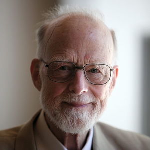
Tony Hoare (born 1934)

Tony Hoare is famous for Hoare Logic, he is a pioneer of process calculi with his Communicating Sequential Processes, and he is the inventor of a famous efficient sorting algorithm called QuickSort. Hoare was the winner of the 1980 Turing Award.

Quicksort

Quicksort is a very early example where recursion is used as the key to a very efficient sorting algorithm. Here is an implementation in Haskell:

> quicksort :: Ord a => [a] -> [a]  
> quicksort [] = []  
> quicksort (x:xs) = 
>    quicksort [ a | a <- xs, a <= x ]  
>    ++ [x]
>    ++ quicksort [ a | a <- xs, a > x ]

The quicksort function has the property that it turns any finite list of items into an ordered list of items.

So in this case the precondition is the property isTrue that holds of any list (in fact of anything at all):

> isTrue :: a -> Bool
> isTrue _ = True

and the postcondition is:

> prop_ordered :: Ord a => [a] -> Bool
> prop_ordered [] = True
> prop_ordered (x:xs) = all (>= x) xs && prop_ordered xs

So we have the following Hoare triple:

{ isTrue xs } ys = quicksort xs { prop_ordered ys }

What this means: if xs is any (finite) list, and ys is the result of the call quicksort xs, then ys is an ordered list.

This Hoare triple for quicksort can be used for automated testing.

Automated test generation

> testR :: Int -> Int -> ([Int] -> [Int])
>                     -> ([Int] -> [Int] -> Bool) -> IO ()
> testR k n f r = if k == n then print (show n ++ " tests passed")
>                 else do
>                   xs <- genIntList
>                   if r xs (f xs) then
>                     do print ("pass on: " ++ show xs)
>                        testR (k+1) n f r
>                   else error ("failed test on: " ++ show xs)

Here is a function for running 100 tests with a given postcondition.

> testPost :: ([Int] -> [Int]) -> ([Int] -> Bool) -> IO ()
> testPost f p = testR 1 100 f (\_ -> p)

Example use

 testPost quicksort prop_ordered

Let's compare quicksort with the following:

> quicksrt :: Ord a => [a] -> [a]  
> quicksrt [] = []  
> quicksrt (x:xs) = 
>    quicksrt [ a | a <- xs, a < x ]  
>    ++ [x]
>    ++ quicksrt [ a | a <- xs, a > x ]

We can test this as well:

 testPost quicksrt prop_ordered

Is there a postcondition property that quicksort has but quicksrt lacks?

> samelength :: [Int] -> [Int] -> Bool
> samelength xs ys = length xs == length ys

> testRel :: ([Int] -> [Int]) -> ([Int] -> [Int] -> Bool) -> IO ()
> testRel f r = testR 1 100 f r

Use this as follows:

testRel quicksrt samelength

It is also possible to use QuickCheck:

 *FSA2> quickCheck (\ xs -> samelength xs (quicksrt xs))
 *** Failed! Falsifiable (after 6 tests):                  
 [-3,-3]

Note: QuickCheck also shrinks the counterexample.

Think of some more properties and relations that can be used to test quicksort and quicksrt.

Next, find some relevant properties to test reverse.

Precondition strengthening

{ p } f { q }

holds, and p' is a property that is stronger than p, then

{ p' } f { q }

holds as well. This is called precondition strenghtening. In order to see what this principle means, we need a good understanding of the relation stronger than.

A property that is stronger than isTrue is the property of being different from the empty list. In Haskell, we can express this as not.null.

Thus, precondition strengthening allows us to derive the following Hoare triple:

{ not.null xs } ys = quicksort xs { sorted ys }

Postcondition weakening

{ p } f { q }

holds, and q' is a property that is weaker than q, then

{ p } f { q' }

holds as well. This is called postcondition weakening. Again, to understand what this means we need a good understanding of what weaker than means.

Hoare triples as contracts

Hoare triples can be viewed as a special case of the contracts used as specifications in design by contract software development.

The preconditions specify what the contract expects. In the case of quicksort, the contract expects nothing. The postconditions express what the contract guarantees. In the case of quicksort, the contract guarantees that the output of the program is an ordered list.

Useful logic notation

> forall = flip all

> infix 1 --> 
> 
> (-->) :: Bool -> Bool -> Bool
> p --> q = (not p) || q

Stronger and Weaker as Predicates on Test Properties

Stronger than$ and weaker than* are relations on the class of test properties.

Implementations of these must assume that we restrict to a finite domain given by a [a].

> stronger, weaker :: [a] -> 
>        (a -> Bool) -> (a -> Bool) -> Bool
> stronger xs p q = forall xs (\ x -> p x --> q x)
> weaker   xs p q = stronger xs q p

Note the presence of [a] for the test domain.

The Weakest and the Strongest Property

Use $\top$ for the property that always holds. This is the weakest possible property. Implementation: \ _ -> True. See isTrue above.

Use $\bot$ for the property that never holds. This is the strongest property. Implementation: \ _ -> False.

Everything satisfies \ _ -> True.

Nothing satisfies \ _ -> False.

Negating a Property

> neg :: (a -> Bool) -> a -> Bool
> neg p = \ x -> not (p x)

But there is a simpler version:

(not.) = \ p -> not . p =  \ p x -> not (p x)

Conjunctions and Disjunctions of Properties

> infixl 2 .&&. 
> infixl 2 .||.

> (.&&.) :: (a -> Bool) -> (a -> Bool) -> a -> Bool
> p .&&. q = \ x -> p x && q x 
> 
> (.||.) :: (a -> Bool) -> (a -> Bool) -> a -> Bool
> p .||. q = \ x -> p x || q x

Review questions: What is the difference between (&&) and .(&&). ? What is the difference between (||) and .(||). ?

Examples

*FSA2> stronger [0..10] even (even .&&. (>3))
False
*FSA2> stronger [0..10] even (even .||. (>3))
True
*FSA2> stronger [0..10] (even .&&. (>3)) even
True
*FSA2> stronger [0..10] (even .||. (>3)) even
False

Further exercises with this: left to you.

The following code can be useful:

> compar :: [a] -> (a -> Bool) -> (a -> Bool) -> String
> compar xs p q = let pq = stronger xs p q 
>                     qp = stronger xs q p 
>                 in 
>                   if pq && qp then "equivalent"
>                   else if pq  then "stronger"
>                   else if qp  then "weaker"
>                   else             "incomparable"

Importance of Precondition Strengthening for Testing

If you strengthen the requirements on your inputs, your testing procedure gets weaker.

Reason: the set of relevant tests gets smaller.

Note: the precondition specifies the relevant tests.

Preconditions should be as weak as possible (given a function and a postcondition).

Importance of Postcondition Weakening for Testing

If you weaken the requirements on your output, your testing procedure gets weaker.

Reason: the requirements that you use for checking the output get less severe.

Note: the postcondition specifies the strength of your tests.

Postconditions should be as strong as possible (given a function and a precondition).

Falsifiability, Critical Rationalism, Open Society

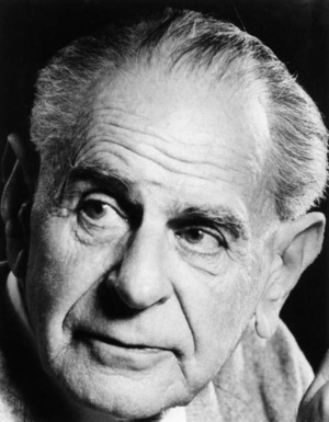
Karl Popper (1902--1992)

To say something meaningful, say something that can turn out false.

Application to Hoare Reasoning

A Hoare triple is an implication, with the precondition in a negative position, and the postcondition in a positive position.

To strengthen a Hoare triple (make the specification of a function more meaningful), one should make the precondition as weak as possible and the postcondition as strong as possible.

Pre- and Postcondition Composition Rule

From

{ p } f { q }     and    { q } g { r }

conclude:

{ p } g . f { r }

This gives an important way to derive useful specifications for compositions from specifications for their parts.

Function Composition, With Flipped Order

(.) :: (a -> b) -> (c -> a) -> (c -> b)
f . g = \ x -> f (g x)

> infixl 2 #
> 
> (#) :: (a -> b) -> (b -> c) -> (a -> c)
> (#) = flip (.)

Read f # g as f followed by g.

Restatement of the composition rule

From

{ p } f { q }     and    { q } g { r }

conclude:

{ p } f # g { r }

Function Application, with Flipped Order

> infixl 1 $$
> 
> ($$) :: a -> (a -> b) -> b
> ($$) = flip ($)

Example:

*FSA2> 5 $$ succ
6

Review Question: can you work out the types and the definitions of flip and $?

Review Question: why is $ a useful operation?

No Assignment in Pure Functional Programming

Question: what is the difference between $\lambda x \mapsto x+1$ and the assignment statement $x := x+1$?

Answer: for one thing, the types are different:

$\lambda x \mapsto x+1$ is a function.

$x := x+1$ is interpreted in the context of a current memory allocation (an environment), with $x$ naming a memory cell.

\[ \begin{array}{ccccc} \cdots & x & y & z & \cdots \\ \cdots & \Box & \Box & \Box & \cdots \end{array} \]

Environments

An environment (for integers, say), is a function of type $V \to Int$, where $V$ is a set of variables.

Assignment as Update

Assignment can be viewed as updating the definition of a function.

> update :: Eq a => (a -> b) -> (a,b) -> a -> b
> update f (x,y) = \ z -> if x == z then y else f z

> updates :: Eq a => (a -> b) -> [(a,b)] -> a -> b
> updates = foldl update

The command $x := x+1$ is an update operation on an environment.

Variables, Environments, Expressions

> type Var = String
> type Env = Var -> Integer

To implement variable assignment we need a datatype for expressions, for the assign command assigns an expression to a variable.

> data Expr = I Integer | V Var
>           | Add Expr Expr 
>           | Subtr Expr Expr 
>           | Mult Expr Expr 
>           deriving (Eq,Show)

Evaluation of an expression in an environment

> eval :: Expr -> Env -> Integer 
> eval (I i) _ = i 
> eval (V name) env = env name
> eval (Add e1 e2) env = (eval e1 env) + (eval e2 env)
> eval (Subtr e1 e2) env = (eval e1 env) - (eval e2 env)
> eval (Mult e1 e2) env = (eval e1 env) * (eval e2 env)

Variable Assignment in an Environment

> assign :: Var -> Expr -> Env -> Env 
> assign var expr env =  update env (var, eval expr env)

Environment initialisation

An environment is a finite object, so it will yield $\bot$ (undefined) for all but a finite number of variables.

The initial environment is everywhere undefined:

> initEnv :: Env 
> initEnv = \ _ -> undefined

Simple example

 initialize an environment; 
 x := 3; 
 y := 5; 
 z := x*y; 
 evaluate z

> example = initEnv $$ 
>           assign "x" (I 3) # 
>           assign "y" (I 5) # 
>           assign "z" (Mult (V "x") (V "y")) #
>           eval (V "z")

 *FSA2> :t example
 example :: Int
 *FSA2> example
 15

The Four Ingredients of Imperative Programming

Variable Assignment: <var> := <expr>
Conditional Execution: if <bexpr> then <statement1> else <statement2>
Sequential Composition: <statement1> ; <statement2>
Iteration: while <expr> do <statement>

These four ingredients make for a Turing complete programming language. A programming language is Turing complete if it is powerful enough to simulate a single taped Turing machine.

It is believed that such languages can express any function that can be computed by an algorithm. This article of faith is called the Church-Turing thesis.

Implementation of While Language in Haskell

Conditions:

> data Condition = Eq Expr Expr 
>                | Lt Expr Expr 
>                | Gt Expr Expr 
>                | Ng Condition 
>                | Cj [Condition] 
>                | Dj [Condition]
>                deriving (Eq,Show)

Statements:

> data Statement = Ass Var Expr
>                | Cond Condition Statement Statement
>                | Seq [Statement]
>                | While Condition Statement
>                deriving (Eq,Show)

Condition Evaluation

> evalc :: Condition -> Env -> Bool
> evalc (Eq e1 e2) env = eval e1 env == eval e2 env
> evalc (Lt e1 e2) env = eval e1 env <  eval e2 env
> evalc (Gt e1 e2) env = eval e1 env >  eval e2 env 
> evalc (Ng c) env = not (evalc c env)
> evalc (Cj cs) env = and (map (\ c -> evalc c env) cs)
> evalc (Dj cs) env = or  (map (\ c -> evalc c env) cs)

Statement Execution

Executing a statement of the While language should be an operation that maps environments to environments.

> exec :: Statement -> Env -> Env 
> exec (Ass v e) env = assign v e env
> exec (Cond c s1 s2) env = 
>  if evalc c env then exec s1 env else exec s2 env 
> exec (Seq ss) env = foldl (flip exec) env ss 
> exec w@(While c s) env = 
>  if not (evalc c env) then env 
>  else exec w (exec s env)

Example

fib n
x := 0; y := 1; 
while n > 0 do { z := x; x := y; y := z+y; n := n-1 }

> fib :: Statement
> fib = Seq [Ass "x" (I 0), Ass "y" (I 1), 
>            While (Gt (V "n") (I 0))
>              (Seq [Ass "z" (V "x"), 
>                    Ass "x" (V "y"),
>                    Ass "y" (Add (V "z") (V "y")), 
>                    Ass "n" (Subtr (V "n") (I 1))])]

> run :: [(Var,Integer)] -> Statement -> [Var] -> [Integer]
> run xs program vars = 
>   exec program (updates initEnv xs) $$ 
>     \ env -> map (\ c -> eval c env) (map V vars)

Call this with

run [("n",1000)] fib ["x"]

Comparison with Functional Version

In order to get a close connection, we first take a closer look at while loops.

Do you know the silly joke about the computer scientist who died under the shower? He read the text on the shampoo bottle and followed the instruction:

lather; rinse; repeat

This is an infinite loop. In many cases we need to add a stop condition:

until clean (lather # rinse)

while (not.clean) (lather # rinse)

The until function is predefined in Haskell.

Review question Can you give a type specification of until? Can you give a definition?

Here is a definition of while:

> while :: (a -> Bool) -> (a -> a) -> a -> a
> while = until . (not.)

Check the types!

Famous example:

> euclid m n = (m,n) $$
>    while (\ (x,y) -> x /= y) 
>          (\ (x,y) -> if x > y then (x-y,y) 
>                               else (x,y-x)) #
>          fst

While + Return

Sometimes it is useful to include a function for transforming the result:

> whiler :: (a -> Bool) -> (a -> a) -> (a -> b) -> a -> b
> whiler p f r = while p f # r

Example:

> euclid2 m n = (m,n) $$
>           whiler (\ (x,y) -> x /= y) 
>                  (\ (x,y) -> if x > y then (x-y,y) 
>                                       else (x,y-x))
>                  fst

Now we can do fib in functional imperative style:

> fibonacci :: Integer -> Integer
> fibonacci n = fibon (0,1,n)
> 
> fibon = whiler 
>          (\ (_,_,n) -> n > 0)
>          (\ (x,y,n) -> (y,x+y,n-1))
>          (\ (x,_,_) -> x)

Also compare:

> fb :: Integer -> Integer
> fb n = fb' 0 1 n where 
>    fb' x y 0 = x 
>    fb' x y n = fb' y (x+y) (n-1)

Clearly, these are all versions of the same algorithm.

Back to Hoare Logic

The Hoare rule for while statements:

From

{ p } f { p }

derive

{ p } while c f { p .&&. not.c }

The property p in statement { p } f { p } is called a loop invariant.

For connections between Hoare Logic and modal logics such as PDL see (Eijck and Stokhof 2006).

The key to showing the correctness of the imperative version of the Fibonacci algorithm is to show that (x,y) = (F(N-n),F(N-n+1)) holds for the step inside the while loop, where N is the initial value of variable n.

In other words, suppose (x,y) = (F(N-n),F(N-n+1)), and execute the statement (x,y,n) := (y,x+y,n-1). Then afterwards, (x,y) = (F(N-n),F(N-n+1)) holds again.

The functional programmer, instead of checking a loop invariant, proves with induction on k that after the call fb n, fb' is always called with parameters F(n-k), F(n-k+1), k.

We see that proving the loop invariant corresponds to proving the inductive step in the induction proof. In the imperative version we have to deal with three variables x,y,n and in the recursive functional version we reason about three function arguments.

Appendix: How Much Does a Test Reveal?

You have 27 coins and a balance scale. All coins have the same weight, except for one coin, which is counterfeit: it is lighter than the other coins.

How many weighing tests are needed to find the light coin?
And how do you do it?
Can you show that a more efficient method (using fewer tests) is impossible?

Implementation of a balance scale

A balance scale gives three possible outcomes:

Left scale is lighter
Left scale is heavier
The two scales are in balance.

> data Coin = C Int
> 
> w :: Coin -> Float 
> w (C n) = if n == lighter then 1 - 0.01
>           else if n == heavier then 1 + 0.01
>           else 1
> 
> weight :: [Coin] -> Float
> weight = sum . (map w)
> 
> balance :: [Coin] -> [Coin] -> Ordering 
> balance xs ys = 
>   if weight xs < weight ys then LT
>   else if weight xs > weight ys then GT
>   else EQ

Using the Balance

*FSA2> balance [C 1] [C 2] 
EQ
*FSA2> balance [C 1, C 2] [C 3, C 4]
GT

Solution

 *FSA2> balance [C i | i <- [1..9]] [ C i | i <- [10..18]] 
 LT
 *FSA2> balance [C i | i <- [1..3]] [ C i | i <- [4..6]] 
 LT
 *FSA2> balance [C 1] [C 2]
 EQ

So C 3 is the counterfeit coin.

Second Testing Challenge

This time you have 3 coins and a balance. Two coins have the same weight, but there is one coin which has different weight from the other coins.

How many weighing tests are needed to find the odd coin?
And how do you do it?
Can you show that a more efficient method (using fewer tests) is impossible?

Third Testing Challenge

This time you have 12 coins and a balance. All coins have the same weight, except for one coin which has different weight from the other coins.

How many weighing tests are needed to find the odd coin?
And how do you do it?
Can you show that a more efficient method (using fewer tests) is impossible?

Some General Questions

Using a balance can be viewed as a test with three possible outcomes. If you perform $n$ balance tests, how much information does that give you (at most)?
How much information is required to pick out an odd coin (lighter or heavier) from among $n$ other coins? What can you conclude?
If you perform $n$ tests, each of which has $m$ possible outcomes, how much information does your testing activity give you?

Note

Iteration (using while and repeat loops) versus recursion is the topic of chapter 2 of the classic (Aho and Ullman 1994). This book is freely available on internet; you can find it here. Chapter 2 is here.

Lab work week 2

Back to main course page

Aho, Alfred V., and Jeffrey D. Ullman. 1994. Foundations of Computer Science — C Edition. W. H. Freeman.

Eijck, J. van, and M. Stokhof. 2006. “The Gamut of Dymamic Logics.” In The Handbook of the History of Logic, edited by D.M. Gabbay and J. Woods, 7 — Logic and the Modalities in the Twentieth Century:499–600. Elsevier.