Recently, the use of mathematical concept analysis has been proposed as an alternative to the use of cluster analysis for the purpose of legacy code analysis [35,48,50,51]. As has been argued in [21], concept analysis avoids some of the problems encountered when using cluster analysis for the purpose of object identification.
Concept analysis starts with a table indicating the features of a given set of items. It then builds up so-called concepts which are maximal sets of items sharing certain features. All possible concepts can be grouped into a single lattice, the so-called concept lattice. The smallest concepts consist of few items having potentially many different features, the largest concepts consist of many different items that have only few features in common.
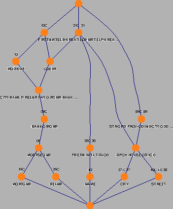
An example concept lattice is shown in Figure 2. This lattice was derived automatically from a 100,000 LOC COBOL case study. The items in this lattice are fields of records that are read from or written to file. They are shown as names below each concept in Figure 2. The features are based on the use of fields in programs: If a field (or in fact, the type inferred for that field) is used in a given program, this program becomes a feature of that field. The programs are written above each concept in Figure 2. Each concept in that figure corresponds to a combination of fields and the programs using them, as occurring in the legacy system. Each concept is a candidate class. Connections between classes correspond to aggregation, association, or inheritance.
To see how the lattice of Figure 2 can help to find objects, let us browse through some of the concepts. The row just above the bottom element consists of five separate concepts, each containing a single field. As an example, the leftmost concept deals with mortgage numbers stored in the field MORTGNR. With it is associated program 19C, which according to the comment lines at the beginning of this program performs certain checks on the validity of mortgage numbers. This program only uses the field MORTGNR, and no other ones. As another example, the concept STREET (at the bottom right) has three different programs directly associated with it. Of these, 40 and 40C compute a certain standardized extract from a street, while program 38 takes care of standardizing street names.
If we move up in the lattice, the concepts become larger, i.e., contain more items. The leftmost concept at the second row contains three different fields: the mortgage sequence number MORTSEQNR written directly at the node, as well as the two fields from the lower concepts connected to it, MORTGNR and RELNR. Program 09 uses all three fields to search for full mortgage and relation records.
Another concept of interest is the last one of the second row. It represents the combination of the fields ZIPCD (zip code), HOUSE (house number), and CITYCD (city code), together with STREET and CITY. This combination of five is a separate concept, because it actually occurs in four different programs (89C, 89, 31C, 31). However, there are no programs that only use these variables, and hence this concept has no program associated with it. It corresponds to a common superclass for both the 89C,89 and the 31,31C concepts.
In short, the lattice provides insight into the organization of the legacy system, and gives suggestions for grouping programs and fields into classes. The human re-engineer can use this information to select initial candidate classes based on the data and functionality available in the legacy.
The crucial step with both cluster and concept analysis is to apply the correct filtering criteria, in order to reduce the overwhelming number of variables, sections, programs, databases, and so on, to the relevant ones. Such selection criteria may differ from system to system, and can only be found by trying several alternatives on the system being investigated--this is exactly where the system understanding tool set discussed in Section 2.2 comes in. The selection criteria used to arrive at Figure 2 are based on persistent data and metrics derived from the call relation, as discussed in [20,21].